


radis package
Subpackages
- radis.api package
- Submodules
- radis.api.atomic_pf_api module
- radis.api.cache_files module
- radis.api.cdsdapi module
- radis.api.dbmanager module
- radis.api.exomolapi module
MdbExomolcheck_code_level()compute_wavenumber_ranges()exact_molname_exomol_to_simple_molname()get_exomol_database_list()get_exomol_full_isotope_name()get_list_of_known_isotopes()make_j2b()make_j2b_m0()make_jj2b()pickup_gE()read_broad()read_def()read_pf()read_states()read_trans()wavenumber_range_HDO_VTT()wavenumber_tag()
- radis.api.geisaapi module
- radis.api.hdf5 module
- radis.api.hitempapi module
HITEMPDatabaseManagerdecrypt_password()download_and_decompress_CO2_into_df()download_hitemp_file()encrypt_password()get_encryption_key()get_last()get_recent_hitemp_database_year()keep_only_relevant()login_to_hitran()parse_one_CO2_block()read_and_write_chunked_for_CO2()read_config()register_partial_hitemp_co2()running_in_spyder()setup_credentials()store_credentials()
- radis.api.hitranapi module
- radis.api.kuruczapi module
- radis.api.nistapi module
- radis.api.tools module
- Module contents
- Submodules
- radis.db package
- Subpackages
- Submodules
- radis.db.classes module
- Summary
- Molecules
- Routine Listing
EXOMOL_ONLY_ISOTOPES_NAMESElectronicStateHITRAN_CLASS1HITRAN_CLASS10HITRAN_CLASS2HITRAN_CLASS3HITRAN_CLASS4HITRAN_CLASS5HITRAN_CLASS6HITRAN_CLASS7HITRAN_CLASS8HITRAN_CLASS9HITRAN_GROUP1HITRAN_GROUP2HITRAN_GROUP3HITRAN_GROUP4HITRAN_GROUP5HITRAN_GROUP6HITRAN_MOLECULESIsotopeMoleculeget_element_symbol()get_ielem_charge()get_molecule()get_molecule_identifier()int_to_roman()is_atom()is_neutral()roman_to_int()to_conventional_name()
- radis.db.conventions module
- radis.db.degeneracies module
- radis.db.hitemp_co2 module
- radis.db.molecules module
- radis.db.molparam module
- radis.db.references module
- radis.db.utils module
- radis.db.classes module
- Module contents
- radis.io package
- radis.lbl package
- Submodules
- radis.lbl.bands module
- radis.lbl.base module
- radis.lbl.broadening module
- Summary
- Routine Listing
BroadenFactorydoppler_broadening_HWHM()gamma_vald3()gaussian_FT()gaussian_lineshape()lorentzian_FT()lorentzian_lineshape()olivero_1977()pressure_broadening_HWHM()project_lines_on_grid()project_lines_on_grid_noneq()voigt_FT()voigt_broadening_HWHM()voigt_lineshape()whiting1968()
- radis.lbl.calc module
- radis.lbl.factory module
- radis.lbl.labels module
- radis.lbl.loader module
- radis.lbl.overp module
- Module contents
LevelsListLevelsList.E_bandsLevelsList.QrefLevelsList.Qvib_refLevelsList.Trot_refLevelsList.Tvib_refLevelsList.bandsLevelsList.bands_refLevelsList.copy_linesLevelsList.cum_weightLevelsList.eq_spectrum()LevelsList.levelsfmtLevelsList.lvl_indexLevelsList.mole_fraction_refLevelsList.non_eq_spectrum()LevelsList.parfuncLevelsList.path_length_refLevelsList.plot_vib_populations()LevelsList.sorted_bandsLevelsList.verboseLevelsList.vib_distribution_refLevelsList.vib_levels
SpectrumFactorySpectrumFactory.NwGSpectrumFactory.NwLSpectrumFactory.SpecDatabaseSpectrumFactory.autoretrievedatabaseSpectrumFactory.autoupdatedatabaseSpectrumFactory.cond_unitsSpectrumFactory.databaseSpectrumFactory.dataframe_engineSpectrumFactory.dataframe_typeSpectrumFactory.df0SpectrumFactory.df1SpectrumFactory.eq_spectrum()SpectrumFactory.eq_spectrum_gpu()SpectrumFactory.eq_spectrum_gpu_interactive()SpectrumFactory.fit_legacy()SpectrumFactory.generate_perf_profile()SpectrumFactory.inputSpectrumFactory.input_wunitSpectrumFactory.interactive_paramsSpectrumFactory.levelsSpectrumFactory.levelspathSpectrumFactory.min_widthSpectrumFactory.miscSpectrumFactory.molparamSpectrumFactory.non_eq_spectrum()SpectrumFactory.optically_thin_power()SpectrumFactory.paramsSpectrumFactory.parsumSpectrumFactory.parsum_calcSpectrumFactory.parsum_tabSpectrumFactory.predict_time()SpectrumFactory.print_perf_profile()SpectrumFactory.profilerSpectrumFactory.reftrackerSpectrumFactory.save_memorySpectrumFactory.truncationSpectrumFactory.unitsSpectrumFactory.verboseSpectrumFactory.warningsSpectrumFactory.wavenumberSpectrumFactory.wavenumber_calcSpectrumFactory.wbroad_centeredSpectrumFactory.woutrange
calc_spectrum()spectrum_test()
- Submodules
- radis.levels package
- radis.los package
- radis.misc package
- Submodules
- radis.misc.arrays module
- Description
anynan()anynan_vaex()arange_len()array_allclose()autoturn()bining()boolean_array_from_ranges()calc_diff()centered_diff()count_nans()evenly_distributed()evenly_distributed_fast()find_first()find_nearest()first_nonnan_index()is_sorted()is_sorted_backward()last_nonnan_index()logspace()nantrapz()non_zero_ranges_in_array()non_zero_values_around()norm()norm_on()numpy_add_at()scale_to()sparse_add_at()
- radis.misc.basics module
all_in()any_in()compare_dict()compare_lists()compare_paths()exec_file()expand_metadata()flatten()in_all()intersect()is_float()is_list()is_number()is_range()key_max_val()list_if_float()make_folders()merge_lists()merge_rename_columns()partition()print_series()remove_duplicates()round_off()stdpath()str2bool()to_str()transfer_metadata()
- radis.misc.config module
- Summary
- Routine Listing
DBFORMATDBFORMATJSONaddDatabankEntries()addDatabankEntries_configformat()convertRadisToJSON()createConfigFile()diffDatabankEntries()getDatabankEntries()getDatabankEntries_configformat()getDatabankList()getDatabankList_configformat()get_config()get_user_config()get_user_config_configformat()init_radis_json()printDatabankEntries()printDatabankEntries_configformat()printDatabankList()printDatabankList_configformat()
- radis.misc.curve module
- radis.misc.database_progress module
- radis.misc.debug module
- radis.misc.log module
- radis.misc.plot module
- radis.misc.printer module
- radis.misc.profiler module
- radis.misc.progress_bar module
- radis.misc.signal module
- radis.misc.utils module
- radis.misc.warning module
AccuracyErrorAccuracyWarningCollisionalBroadeningWarningDatabaseAlreadyExistsDatabaseNotFoundErrorDeprecatedFileWarningElectronicSpectraWarningEmptyDatabaseErrorEmptyDatabaseWarningGPUInitWarningGaussianBroadeningWarningHighTemperatureWarningInconsistentDatabaseErrorInputConditionsWarningIrrelevantFileWarningLinestrengthCutoffWarningMemoryUsageWarningMissingDiluentBroadeningTdepWarningMissingDiluentBroadeningWarningMissingPressureShiftWarningMissingReferenceWarningMissingSelfBroadeningTdepWarningMissingSelfBroadeningWarningMoleFractionErrorNegativeEnergiesWarningNoGPUWarningOutOfBoundErrorOutOfBoundWarningOutOfRangeLinesWarningPerformanceWarningSlitDispersionWarningUnevenWaverangeWarningVoigtBroadeningWarningWarningClassesZeroBroadeningWarningdefault_warning_statusreset_warnings()warn()
- radis.misc.arrays module
- Module contents
DatabankNotFoundDatabaseProgressPrinterDatabaseProgressPrinter.HEADER_WIDTHDatabaseProgressPrinter.complete()DatabaseProgressPrinter.download_progress()DatabaseProgressPrinter.download_summary()DatabaseProgressPrinter.header()DatabaseProgressPrinter.info()DatabaseProgressPrinter.lines_progress()DatabaseProgressPrinter.parsing_progress()DatabaseProgressPrinter.parsing_summary()DatabaseProgressPrinter.progress_bar()DatabaseProgressPrinter.section()DatabaseProgressPrinter.success()DatabaseProgressPrinter.warning()
NotInstalledProgressBararray_allclose()autoturn()bining()calc_diff()centered_diff()compare_dict()compare_lists()compare_paths()count_nans()curve_add()curve_distance()curve_divide()curve_multiply()curve_substract()evenly_distributed()exec_file()export()find_first()find_nearest()getDatabankEntries()getDatabankList()getProjectRoot()get_progress_printer()is_float()is_sorted()is_sorted_backward()key_max_val()list_if_float()logspace()make_folders()merge_lists()nantrapz()norm()norm_on()partition()remove_duplicates()resample()resample_even()scale_to()
- Submodules
- radis.phys package
- Submodules
- radis.phys.air module
- radis.phys.blackbody module
- radis.phys.constants module
- radis.phys.convert module
J2K()J2cm()J2eV()K2J()K2cm()K2eV()atm2bar()atm2torr()bar2atm()bar2torr()cm2J()cm2J_vaex()cm2K()cm2eV()cm2hz()cm2nm()cm2nm_air()dcm2dnm()dcm2dnm_air()dhz2dnm()div_safe()dnm2dcm()dnm2dhz()dnm_air2dcm()eV2J()eV2K()eV2cm()eV2nm()hz2cm()hz2nm()nm2cm()nm2eV()nm2hz()nm_air2cm()torr2atm()torr2bar()zero2nan()
- radis.phys.morse module
- radis.phys.units module
- radis.phys.units_astropy module
- Module contents
- Submodules
- radis.spectrum package
- Submodules
- radis.spectrum.compare module
- radis.spectrum.equations module
- radis.spectrum.models module
- radis.spectrum.operations module
- radis.spectrum.rescale module
get_reachable()get_recompute()get_redundant()non_rescalable_keysordered_keysrescale_abscoeff()rescale_absorbance()rescale_emisscoeff()rescale_emissivity_noslit()rescale_mole_fraction()rescale_path_length()rescale_radiance()rescale_radiance_noslit()rescale_transmittance()rescale_transmittance_noslit()rescale_xsection()update()
- radis.spectrum.spectrum module
- radis.spectrum.utils module
- Module contents
PerfectAbsorber()Radiance()Radiance_noslit()SpectrumSpectrum.conditionsSpectrum.cSpectrum.populationsSpectrum.apply_slit()Spectrum.argmax()Spectrum.argmin()Spectrum.cSpectrum.cite()Spectrum.compare_with()Spectrum.cond_unitsSpectrum.conditionsSpectrum.copy()Spectrum.crop()Spectrum.exit_gpu()Spectrum.fileSpectrum.fit_model()Spectrum.from_array()Spectrum.from_hdf5()Spectrum.from_mat()Spectrum.from_spec()Spectrum.from_specutils()Spectrum.from_txt()Spectrum.from_xsc()Spectrum.generate_perf_profile()Spectrum.get()Spectrum.get_baseline()Spectrum.get_condition()Spectrum.get_conditions()Spectrum.get_integral()Spectrum.get_name()Spectrum.get_populations()Spectrum.get_power()Spectrum.get_quantities()Spectrum.get_radiance()Spectrum.get_radiance_noslit()Spectrum.get_rovib_levels()Spectrum.get_slit()Spectrum.get_vars()Spectrum.get_vib_levels()Spectrum.get_wavelength()Spectrum.get_wavenumber()Spectrum.get_waveunit()Spectrum.gpu_appSpectrum.has_nan()Spectrum.is_at_equilibrium()Spectrum.is_optically_thin()Spectrum.line_survey()Spectrum.linesSpectrum.max()Spectrum.min()Spectrum.nameSpectrum.normalize()Spectrum.offset()Spectrum.plot()Spectrum.plot_populations()Spectrum.plot_slit()Spectrum.populationsSpectrum.print_conditions()Spectrum.print_perf_profile()Spectrum.profilerSpectrum.recalc_gpu()Spectrum.referencesSpectrum.resample()Spectrum.resample_even()Spectrum.rescale_mole_fraction()Spectrum.rescale_path_length()Spectrum.save()Spectrum.savetxt()Spectrum.sort()Spectrum.store()Spectrum.take()Spectrum.to_hdf5()Spectrum.to_json()Spectrum.to_pandas()Spectrum.to_specutils()Spectrum.trim()Spectrum.unitsSpectrum.update()
Transmittance()Transmittance_noslit()calculated_spectrum()experimental_spectrum()get_diff()get_distance()get_ratio()get_residual()get_residual_integral()plot_diff()transmittance_spectrum()
- Submodules
- radis.test package
- radis.tools package
- Submodules
- Module contents
Module contents
       *(((((((
        ((((((((((((              ,(((((
        ((((((((((((((((/   *((((((((((*
         ((((((((((((((((( ((((((((((((
             (((((((( (((((((((((((
                *
              @@  *@@       ..  /@@
         @@&  @@  *@@       @@  /@@  @@%
     @@  @@&  @@  *@@  @@&  @@  /@@  @@%  @@
     @@  @@&  @@  *@@  @@&  @@  /@@  @@%  @@
     @@  @@&  @@  *@@  @@&  @@  /@@  @@%  @@  (@
,@   @@  @@&  @@  *@@  @@&  @@  /@@  @@%  @@
@@   @@  @@&  @@  ,.
                           ,%&&&&&&&&&&&&&&&&&&&
 &&&&&&&&&&&&&&&&&&&&&&&&&&&&&&&&&&&&&&&&&&&&&
  &&&&&&&&&&&&&&&&&&&&&&&&&&&&&&&&&&&&&&&&&&&
    &&&&&&&&&&&&&&&&@@@@@@&@@@&&&@@@&&&&&&&&
      &&&&&&&&&&&&&&&@@@@@@&&&&&&&&&&&&&&&
        &&&&&&&&&&&&&&&&&&&&&&&&&&&&&&&&
          &&&&&&&&&&&&&&&&&&&&&&&&&&&.
              &&&&&&&&&&&&&&&&&&&
                      .**.
                       &&&,
                        &&
- class LevelsList(parfunc, bands, levelsfmt, sortby='Ei', copy_lines=False, verbose=True)[source]
Bases:
objectA class to generate a Spectrum from a list of precalculated bands at a given reference temperature.
Warning
only valid under optically thin conditions!!
- eq_spectrum(Tgas, overpopulation=None, mole_fraction=None, path_length=None, save_rescaled_bands=False)[source]
See
eq_spectrum()Warning
only valid under optically thin conditions!!
- Parameters:
… same as usually. If None, then the reference value (used to
calculate bands) is used
- Other Parameters:
save_rescaled_bands (boolean) – save updated bands. Take some time as it requires rescaling all bands individually (which is only done on the MergedSlabs usually) Default
False
- non_eq_spectrum(Tvib=None, Trot=None, Ttrans=None, vib_distribution='boltzmann', overpopulation=None, mole_fraction=None, path_length=None, save_rescaled_bands=False)[source]
-
Warning
only valid under optically thin conditions!!
- Parameters:
… same as usually. If None, then the reference value (used to
calculate bands) is used
- Other Parameters:
save_rescaled_bands (boolean) – save updated bands. Take some time as it requires rescaling all bands individually (which is only done on the MergedSlabs usually) Default
False
Notes
Implementation:
Generation of a new spectrum is done by recombination of the precalculated bands with
- plot_vib_populations(nfig=None, **kwargs)[source]
Plot current distribution of vibrational levels.
By constructions populations are shown as divided by the state degeneracy, i.e, g = gv * (2J+1) * gi * gs
- Parameters:
nfig (str, int) – name of Figure to plot on
kwargs (**dict) – arguments are forwarded to plot()
- MergeSlabs(*slabs: Spectrum, **kwargs: dict) Spectrum[source]
Combines several slabs into one. Useful to calculate multi-gas slabs. Linear absorption coefficient is calculated as the sum of all linear absorption coefficients, and the RTE is recalculated to get the total radiance. You can also simply use:
s1//s2
Merged spectrum
1+2is calculated with Eqn (4.3) of the [RADIS-2018] article, generalized to N slabs :\[ \begin{align}\begin{aligned}j_{\lambda, 1+2} = j_{\lambda, 1} + j_{\lambda, 2}\\k_{\lambda, 1+2} = k_{\lambda, 1} + k_{\lambda, 2}\end{aligned}\end{align} \]where
\[j_{\lambda}, k_{\lambda}\]are the emission coefficient and absorption coefficient of the two slabs
1and2. Emission and absorption coefficients are calculated if not given in the initial slabs (if possible).- Parameters:
slabs (list of Spectra, each representing a slab) –
path_lengthmust be given in Spectrum conditions, and equal for all spectra.line-of-sight:
slabs
            [0]        \====
light       [1]  ->     )===  observer
            [n]        /====
- Other Parameters:
kwargs input
resample (
'never','intersect','full') – what to do when spectra have different wavespaces:If
'never', raises an errorIf
'intersect', uses the intersection of all ranges, and resample spectra on the most resolved wavespace.If
'full', uses the overlap of all ranges, resample spectra on the most resolved wavespace, and fill missing data with 0 emission and 0 absorption
Default
'never'out (
'transparent','nan','error') – what to do if resampling is out of bounds:'transparent': fills with transparent medium.'nan': fills with nan.'error': raises an error.
Default
'nan'optically_thin (boolean) – if
True, merge slabs in optically thin mode. DefaultFalseverbose (boolean) – if
True, print messages and warnings. DefaultFalsemodify_inputs (False) – if
True, slabs are modified directly when they are resampled. This avoids making a copy so is slightly faster. DefaultFalse.
- Returns:
Spectrum – observed at the output. Conditions and units are transported too, unless there is a mismatch then conditions are dropped (and units mismatch raises an error because it doesnt make sense)
- Return type:
object representing total emission and total transmittance as
Examples
Merge two spectra calculated with different species (physically correct only if broadening coefficients dont change much):
from radis import calc_spectrum, MergeSlabs
s1 = calc_spectrum(...)
s2 = calc_spectrum(...)
s3 = MergeSlabs(s1, s2)
The last line is equivalent to:
s3 = s1//s2
Load a spectrum precalculated on several partial spectral ranges, for a same molecule (i.e, partial spectra are optically thin on the rest of the spectral range):
from radis import load_spec, MergeSlabs
spectra = []
for f in ['spec1.spec', 'spec2.spec', ...]:
    spectra.append(load_spec(f))
s = MergeSlabs(*spectra, resample='full', out='transparent')
s.update()   # Generate missing spectral quantities
s.plot()
- PerfectAbsorber(s: Spectrum) Spectrum[source]
Makes a new Spectrum with the same transmittance/absorbance as Spectrum
s, but with radiance set to 0. Useful to get contribution of different slabs in line-of-sight calculations (see example).- Parameters:
s (Spectrum) –
Spectrumobject- Returns:
s_tr –
Spectrumobject, with only thetransmittance,absorbanceand/orabscoeffpart ofs, whereradiance_noslit,emisscoeffandemissivity_noslit(if they exist) have been set to 0- Return type:
Examples
Let’s say you have a total line of sight:
s_los = s1 > s2 > s3
If you now want to get the contribution of
s2to the line-of-sight emission, you can do:(s2 > PerfectAbsorber(s3)).plot('radiance_noslit')
And the contribution of
s1would be:(s1 > PerfectAbsorber(s2>s3)).plot('radiance_noslit')
See more examples in Line-of-Sight module
- Radiance(s: Spectrum) Spectrum[source]
Returns a new Spectrum with only the
radiancecomponent ofs- Parameters:
s (Spectrum) –
Spectrumobject- Returns:
s_tr –
Spectrumobject, with onlyradiancedefined- Return type:
Examples
This function is useful to use Spectrum algebra operations:
s = calc_spectrum(...)   # contains emission & absorption arrays
rad = Radiance(s)        # contains radiance array only
rad -= 0.1    # arithmetic operation is applied to Radiance only
Equivalent to:
rad = s.take('radiance')
See also
Radiance_noslit(),Transmittance_noslit(),Transmittance(),take()
- Radiance_noslit(s: Spectrum) Spectrum[source]
Returns a new Spectrum with only the
radiance_noslitcomponent ofs- Parameters:
s (Spectrum) –
Spectrumobject- Returns:
s_tr –
Spectrumobject, with onlyradiance_noslitdefined- Return type:
Examples
This function is useful to use Spectrum algebra operations:
s = calc_spectrum(...)   # contains emission & absorption arrays
rad = Radiance_noslit(s) # contains 'radiance_noslit' array only
rad -= 0.1    # arithmetic operation is applied to Radiance_noslit only
Equivalent to:
rad = s.take('radiance_noslit')
See also
- SerialSlabs(*slabs: Spectrum, **kwargs: dict) Spectrum[source]
Adds several slabs along the line-of-sight. If adding two slabs only, you can also use:
s1>s2
Serial spectrum
1>2is calculated with Eqn (4.2) of the [RADIS-2018] article, generalized to N slabs :\[ \begin{align}\begin{aligned}I_{\lambda, 1>2} = I_{\lambda, 1} \tau_{\lambda, 2} + I_{\lambda, 2}\\\tau_{\lambda, 1+2} = \tau_{\lambda, 1} \cdot \tau_{\lambda, 2}\end{aligned}\end{align} \]where
\[I_{\lambda}, \tau_{\lambda}\]are the radiance and transmittance of the two slabs
1and2. Radiance and transmittance are calculated if not given in the initial slabs (if possible).- Parameters:
slabs (list of Spectra, each representing a slab) –
line-of-sight:
slabs       [0]     [1]  ............... [n]
             :       :                    :         \====
light        *   ->  *        ->          *    ->    )===  observer
                                                    /====
resample_wavespace (
'never','intersect','full') – what to do when spectra have different wavespaces:If
'never', raises an errorIf
'intersect', uses the intersection of all ranges, and resample spectra on the most resolved wavespace.If
'full’, uses the overlap of all ranges, resample spectra on the most resolved wavespace, and fill missing data with 0 emission and 0 absorption
Default
'never'out (
'transparent','nan','error') – what to do if resampling is out of bounds:'transparent': fills with transparent medium.'nan': fills with nan.'error': raises an error.
Default
'nan'
- Other Parameters:
verbose (bool) – if
True, more blabla. DefaultFalsemodify_inputs (False) – if
True, slabs wavelengths/wavenumbers are modified directly when they are resampled. This avoids making a copy so it is slightly faster. DefaultFalse.Note
for large number of slabs (in radiative transfer calculations) you surely want to use this option !
- Returns:
Spectrum – observed at the output (slab[n+1]). Conditions and units are transported too, unless there is a mismatch then conditions are dropped (and units mismatch raises an error because it doesnt make sense)
- Return type:
object representing total emission and total transmittance as
Examples
Add s1 and s2 along the line of sight: s1 –> s2:
s1 = calc_spectrum(...)
s2 = calc_spectrum(...)
s3 = SerialSlabs(s1, s2)
The last line is equivalent to:
s3 = s1>s2
- class SpecDatabase(path='.', filt='.spec', add_info=None, add_date='%Y%m%d', verbose=True, binary=True, nJobs=-2, batch_size='auto', lazy_loading=True, update_register_only=False)[source]
Bases:
SpecListA Spectrum Database class to manage them all.
It basically manages a list of Spectrum JSON files, adding a Pandas dataframe structure on top to serve as an efficient index to visualize the spectra input conditions, and slice through the Dataframe with easy queries
Similar to
SpecList, but associated and synchronized with a folder- Parameters:
path (str) – a folder to initialize the database
filt (str) – only consider files ending with
filt. Default.specbinary (boolean) – if
True, open Spectrum files as binary files. IfFalseand it fails, try as binary file anyway. DefaultFalse.lazy_loading (bool``) – If
True, load only the data from the summary csv file and the spectra will be loaded when accessed by the get functions. IfFalse, load all the spectrum files. IfTrueand the summary .csv file does not exist, load all spectra
- Other Parameters:
Input for :class:`~joblib.parallel.Parallel` loading of database
nJobs (int) – Number of processors to use to load a database (useful for big databases). BE CAREFULL, no check is done on processor use prior to the execution ! Default
-2: use all but 1 processors. Use1for single processor.batch_size (int or
'auto') – The number of atomic tasks to dispatch at once to each worker. When individual evaluations are very fast, dispatching calls to workers can be slower than sequential computation because of the overhead. Batching fast computations together can mitigate this. Default:'auto'More information in :class:`joblib.parallel.Parallel`
Examples
>>> db = SpecDatabase(r"path/to/database")     # create or loads database

>>> db.update()  # in case something changed
>>> db.see(['Tvib', 'Trot'])   # nice print in console

>>> s = db.get('Tvib==3000')[0]  # get a Spectrum back
>>> db.add(s)  # update database (and raise error because duplicate!)
Note that
SpectrumFactorycan be configured to automatically look-up and update a database when spectra are calculated.The function to auto retrieve a Spectrum from database on calculation time is a method of DatabankLoader class
You can see more examples on the Spectrum Database section of the website.
See also
load_spec(),store(),Methods,get(),get_closest(),get_unique(),Methods,see(),update(),add(),compress_to(),find_duplicates(),Compare,fit_spectrum()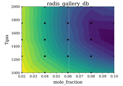
Example #7: Database fitting using SpecDatabase.fit_spectrum
Example #7: Database fitting using SpecDatabase.fit_spectrum- add(spectrum: Spectrum, store_name=None, if_exists_then='increment', **kwargs)[source]
Add Spectrum to database, whether it’s a
Spectrumobject or a file that stores one. Check it’s not in database already.- Parameters:
spectrum (
Spectrumobject, or path to a .spec file (str)) – if aSpectrumobject: stores it in the database (using thestore()method), then adds the file to the database folder. if a path to a file (str): first copy the file to the database folder, then loads the copied file to the database.- Other Parameters:
store_name (
str, orNone) – name of the file where the spectrum will be stored. IfNone, name is generated automatically from the Spectrum conditions (seeadd_info=andif_exists_then=)if_exists_then (
'increment','replace','error','ignore') – what to do if file already exists. If'increment'an incremental digit is added. If'replace'file is replaced (!). If'ignore'the Spectrum is not added to the database and no file is created. If'error'(or anything else) an error is raised. Default'increment'.**kwargs (**dict) – extra parameters used in the case where spectrum is a file and a .spec object has to be created (useless if
spectrumis a file already). kwargs are forwarded to Spectrum.store() method. See thestore()method for more information.Note
Other
store()parameters can be given as kwargs arguments. See below :compress (0, 1, 2) – if
Trueor 1, save the spectrum in a compressed formif 2, removes all quantities that can be regenerated with
update(), e.g, transmittance if abscoeff and path length are given, radiance if emisscoeff and abscoeff are given in non-optically thin case, etc. If not given, use the value ofSpecDatabase.binaryThe performances are usually better if compress = 2. See https://github.com/radis/radis/issues/84.add_info (list) – append these parameters and their values if they are in conditions example:
nameafter = ['Tvib', 'Trot']
discard (list of str) – parameters to exclude. To save some memory for instance Default
['lines', 'populations']: retrieved Spectrum will loose theline_survey()andplot_populations()methods (but it saves a ton of memory!).
Examples
from radis.tools import SpecDatabase
db = SpecDatabase(r"path/to/database")     # create or loads database
db.add(s, discard=['populations'])
You can see more examples on the Spectrum Database section of the website.
See also
- compress_to(new_folder, compress=True, if_exists_then='error')[source]
Saves the Database in a new folder with all Spectrum objects under compressed (binary) format. Read/write is much faster. After the operation, a new database should be initialized in the new_folder to access the new Spectrum.
- Parameters:
new_folder (str) – folder where to store the compressed SpecDatabase. If doesn’t exist, it is created.
compress (boolean, or 2) – if
True, saves under binary format. Faster and takes less space. If2, additionally remove all redundant quantities.if_exists_then (
'increment','replace','error','ignore') – what to do if file already exists. If'increment'an incremental digit is added. If'replace'file is replaced (!). If'ignore'the Spectrum is not added to the database and no file is created. If'error'(or anything else) an error is raised. Default'error'.
See also
- find_duplicates(columns=None)[source]
Find spectra with same conditions. The first duplicated spectrum will be
'False', the following will be'True'(see .duplicated()).- Parameters:
columns (list, or
None) – columns to find duplicates on. IfNone, use all conditions.
Examples
db.find_duplicates(columns={'x_e', 'x_N_II'})

Out[34]:
file
20180710_101.spec    True
20180710_103.spec    True
dtype: bool
You can see more examples in the Spectrum Database section
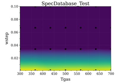
- fit_spectrum(s_exp, residual=None, var=None, normalize=False, normalize_how='max', plot=False, conditions='', **kwconditions)[source]
Returns the Spectrum in the database that has the lowest residual with
s_exp.- Parameters:
s_exp (Spectrum) –
Spectrumto fit (typically: experimental spectrum)- Other Parameters:
var (str) – spectral variable to compare (e.g., ‘radiance’, ‘absorbance’). Required if
s_exphas multiple variables andresidualis not provided.plot (bool) – if
True, plot the residuals against the varying conditions. If one condition varies, a 1D plot is generated. If two conditions vary, a 2D contour plot is generated usingplot_cond(). DefaultFalse.conditions, **kwconditions (str, **dict) – restrain fitting to only Spectrum that match the given conditions in the database. See
get()for more information.normalize (bool, or Tuple) – see
get_residual()normalize_how (‘max’, ‘area’) – see
get_residual()
- Returns:
s_best – closest Spectrum to
s_exp- Return type:
Examples
Compare an experimental spectrum to a database of precomputed spectra:
from radis.tools import SpecDatabase
db = SpecDatabase('path/to/database')
s_best = db.fit_spectrum(s_exp, plot=True)
s_best.plot(nfig='same')
Example #7: Database fitting using SpecDatabase.fit_spectrum
Example #7: Database fitting using SpecDatabase.fit_spectrumUsing a customized residual function (below: to get the transmittance):
from radis import get_residual
db = SpecDatabase('...')
db.fit_spectrum(s_exp, residual=lambda s_exp, s: get_residual(s_exp, s, var='transmittance'))
You can see more examples on the Spectrum Database section More advanced tools for interactive fitting of multi-dimensional, multi-slabs spectra can be found in
fitroom.See also
- interpolate(**kwconditions)[source]
Interpolate existing spectra from the database to generate a new spectrum with conditions kwargs
Examples
db.interpolate(Tgas=300, mole_fraction=0.3)
- to_dict()[source]
Returns all Spectra in database under a dictionary, indexed by file.
- Returns:
out – {path : Spectrum object} dictionary
- Return type:
dict
Note
SpecList.items().values()is equivalent toSpecList.get()
- update(force_reload=False, filt='.spec', update_register_only=False)[source]
Reloads database, updates internal index structure and export it in
<database>.csv.- Parameters:
force_reload (boolean) – if
True, reloads files already in database. DefaultFalsefilt (str) – only consider files ending with
filt. Default.spec
- Other Parameters:
update_register_only (bool) – if
True, load files and update csv but do not keep the Spectrum in memory. DefaultFalse
Notes
Can be loaded in parallel using joblib by setting the
nJobsandbatch_sizeattributes ofSpecDatabase. Seejoblib.parallel.Parallelfor information on the arguments
- class Spectrum(quantities, units=None, conditions=None, cond_units=None, gpu_app=None, populations=None, lines=None, wunit=None, name=None, references={}, check_wavespace=True, **kwargs)[source]
Bases:
objectThis class holds results calculated with the
SpectrumFactorycalculation, with other radiative codes, or experimental data. It can be used to plot different quantities a posteriori, or manipulate output units (for instance convert a spectral radiance per wavelength units to a spectral radiance per wavenumber).See more information on how to generate, edit or combine Spectrum objects on the Spectrum object guide.
- Parameters:
quantities (dict of tuples
{'quantity':(w, a)}or dict{'wavelength/wavenumber': w, quantity': a}) – where quantities are spectral quantities (absorbance, radiance, etc.) and wavenum is in \(cm^{-1}\) or \(nm\) (seewaveunit) Example:# w, k, I are numpy arrays for wavenumbers, absorption coefficient, and radiance. from radis import Spectrum s = Spectrum({"wavenumber":w, "abscoeff":k, "radiance_noslit":I}, wunit='cm-1', units={"radiance_noslit":"mW/cm2/sr/nm", "abscoeff":"cm-1"})
Or:
s = Spectrum({"abscoeff":(w,k), "radiance_noslit":(w,I)},
             wunit="cm-1"
             units={"radiance_noslit":"mW/cm2/sr/nm", "abscoeff":"cm-1"})
See also:
from_array()andfrom_txt()units (dict) – units for quantities
- Other Parameters:
conditions (dict) – physical conditions and calculation parameters
wunit (
'nm','cm-1','nm_vac'orNone) – wavelength in air ('nm'), wavenumber ('cm-1'), or wavelength in vacuum ('nm_vac'). IfNone,'wavespace'must be defined inconditions. Quantities should be evenly distributed along this space for fast convolution with the slit functioncond_units (dict) – units for conditions
- Other Parameters:
name (str, or None) – Give a name to this Spectrum object (automatically used in plots; useful for multislab configurations). Default
Nonepopulations (dict) – a dictionary of all species, and levels. Should be compatible with other radiative codes such as Specair output. Suggested format: {molecules: {isotopes: {elec state: rovib levels}}} e.g:
{'CO2':{1: 'X': df}} # with df a Pandas Dataframe
lines (pandas Dataframe) – all lines in databank (necessary for using
line_survey()). Warning if you want to play with the lines content: The signification of columns inlinesmay be specific to a database format. Plus, some additional columns may have been added by the calculation (e.g:EiandSfor emission integral and linestrength in SpectrumFactory). Refer to the code to know what they mean (and their units)gpu_app (gpuApp) – specifies the gpuApp object that was initialized. this value is auto-generated by SpectrumFactory; don’t provide a manual input. Only not None when spectrum object is produced with one of the GPU methods
eq_spectrum_gpu()oreq_spectrum_gpu_interactive().references (dict) – a dict of
doiof references used to compute this object. Automatically returned with the full bibtex entry bycite()It can also be set a posteriori. Examples = Spectrum() s.references = {"10.1016/j.jqsrt.2010.05.001": "HITEMP-2010 database", "10.1016/j.jqsrt.2018.09.027":["calculation", "post-processing"], # RADIS main paper. Automatically added "10.1016/j.jqsrt.2020.107476":"DIT algorithm"} ) s.cite()
Returns :
Used for DIT algorithm
----------------------
@article{van_den_Bekerom_2021,
    doi = {10.1016/j.jqsrt.2020.107476},
    url = {https://doi.org/10.1016%2Fj.jqsrt.2020.107476},
    year = 2021,
    month = {mar},
    publisher = {Elsevier {BV}},
    volume = {261},
    pages = {107476},
    author = {D.C.M. van den Bekerom and E. Pannier},
    title = {A discrete integral transform for rapid spectral synthesis},
    journal = {Journal of Quantitative Spectroscopy and Radiative Transfer}
}

Used for HITEMP-2010 database
-----------------------------
@article{Rothman_2010,
    doi = {10.1016/j.jqsrt.2010.05.001},
    url = {https://doi.org/10.1016%2Fj.jqsrt.2010.05.001},
    year = 2010,
    month = {oct},
    publisher = {Elsevier {BV}},
    volume = {111},
    number = {15},
    pages = {2139--2150},
    author = {L.S. Rothman and I.E. Gordon and R.J. Barber and H. Dothe and R.R. Gamache and A. Goldman and V.I. Perevalov and S.A. Tashkun and J. Tennyson},
    title = {{HITEMP}, the high-temperature molecular spectroscopic database},
    journal = {Journal of Quantitative Spectroscopy and Radiative Transfer}
}

Used for calculation, post-processing
-------------------------------------
@article{Pannier_2019,
    doi = {10.1016/j.jqsrt.2018.09.027},
    url = {https://doi.org/10.1016%2Fj.jqsrt.2018.09.027},
    year = 2019,
    month = {jan},
    publisher = {Elsevier {BV}},
    volume = {222-223},
    pages = {12--25},
    author = {Erwan Pannier and Christophe O. Laux},
    title = {{RADIS}: A nonequilibrium line-by-line radiative code for {CO}2 and {HITRAN}-like database species},
    journal = {Journal of Quantitative Spectroscopy and Radiative Transfer}
}
</details>
warnings (boolean) – if
True, test if inputs are valid, e.g, spectra are evenly distributed in wavelength, and raise a warning if not. Note that this take ~ 3.5 ms for a 20k points spectrum, when the rest of the creation process is only ~ 1.8ms (makes it 3 times longer, and can be a problem if hundreds of spectra are created in a row). DefaultTrue
Examples
Manipulate a Spectrum calculated by RADIS:
s = calc_spectrum(2125, 2300, Tgas=2000, databank='CDSD')
s.print_conditions()
s.plot('absorbance')
s.line_survey(overlay='absorbance')
s.plot('radiance_noslit', wunits='cm-1', Iunits='W/m2/sr/cm-1')
s.apply_slit(5)
s.plot('radiance')
w, t = s.get('transmittance_noslit')  # for use in multi-slabs configs
Any tuple of numpy arrays (w, I) can also be converted into a Spectrum object from the
Spectrumclass directly, or using thecalculated_spectrum()function. All the following methods are equivalent:from radis import Spectrum, calculated_spectrum s1 = calculated_spectrum(w, I, wunit='nm', Iunit='mW/cm2/sr/nm') s2 = Spectrum.from_array(w, I, 'radiance_noslit', wunit='nm', unit='mW/cm2/sr/nm') s3 = Spectrum({'radiance_noslit': (w, I)}, units={'radiance_noslit':'mW/cm2/sr/nm'}, wunit='nm')
See more examples in the [Spectrum] page.
Spectrum objects can be stored, retrieved, rescaled, resampled:
from radis import load_spec
s = load_spec('co_calculation.spec')
s.rescale_path_length(0.5)                  # calculate for new path_length
s.rescale_mole_fraction(0.02)   # calculate for new mole fraction
s.resample(w_new)               # resample on new wavespace
s.store('co_calculation2.spec')
Notes
Implementation:
quantities are stored in the
self._qdictionary. They are better accessed with theget()method that deals with units and wavespaceWavebase:
- c[source]
convenience wrapper to
conditions:s.c["calculation_time"] is s.conditions["calculation_time"] >> True
- Type:
dict
- populations[source]
Stores molecules, isotopes, electronic states and vibrational or rovibrational populations
- Type:
dict
See also
calculated_spectrum(),transmittance_spectrum(),experimental_spectrum(),from_array(),from_txt(),load_spec()References
[Spectrum]See the Spectrum object page
- apply_slit(slit_function, unit='nm', shape: ['triangular', 'trapezoidal', 'gaussian'] = 'triangular', center_wavespace=None, norm_by='area', mode='valid', plot_slit=False, store=True, slit_dispersion=None, slit_dispersion_threshold=0.01, auto_recenter_crop=True, assert_evenly_spaced=True, verbose=True, inplace=True, *args, **kwargs)[source]
Apply an instrumental slit function to all quantities in Spectrum. Slit function can be generated with usual shapes (see
shape=) or imported from an experimental slit function (path to a text file or numpy array of shape n*2). Convoluted spectra are cut on the edge compared to non-convoluted spectra, to remove side effects. Seemode=to change this behaviour.Warning with units: read about
'unit'and'return_unit'parameters.- Parameters:
slit_function (float or str or array) –
- If
float: generate slit function with FWHM of slit function (in nm or cm-1 depending on
unit=). A (top, base) tuple of (float,float) is required when asking for a trapezoidal slit function.- If
.txt: import experimental slit function from .txt file: format must be 2-columns with wavelengths and intensity (doesn’t have to be normalized)
- If
array: format must be 2-columns with wavelengths and intensity (doesn’t have to be normalized) It is recommended to truncate the input slit function to its minimum useful spectral extension (see Notes of
convolve_with_slit()).
- If
unit (
'nm'or'cm-1') – unit of slit_function (FWHM, or imported file)shape (
'triangular','trapezoidal','gaussian', or any ofSLIT_SHAPES) –- which shape to use when generating a slit. Will call,
respectively,
triangular_slit(),trapezoidal_slit(),gaussian_slit(). Default ‘triangular’
center_wavespace (float, or
None) – center of slit when generated (in unit). Not used if slit is imported.norm_by (
'area','max') – normalisation type: -'area'normalizes the slit function to an areaof 1. It conserves energy, and keeps the same units.
'max'normalizes the slit function to a maximum of 1. The convoluted spectrum units change (they are multiplied by the spectrum waveunit, e.g: a radiance non convoluted in mW/cm2/sr/nm on a wavelength (nm). range will yield a convoluted radiance in mW/cm2/sr. Note that the slit is set to 1 in the Spectrum wavespace (i.e: a Spectrum calculated in cm-1 will have a slit set to 1 in cm-1).
Default
'area'mode (
'valid','same') –'same'returns output of same length as initial spectra,but boundary effects are still visible.
'valid'returns output of length len(spectra) - len(slit) + 1, for which lines outside of the calculated range have no impact. Default'valid'.
- Other Parameters:
assert_evenly_spaced (boolean, or
'resample') – for the convolution to be accurate,wshould be evenly spaced. Ifassert_evenly_spaced=True, then we check this is the case, and raise an error if arrays is not evenly spaced. If'resample', then we resamplewandIif needed. Recommended, but it takes some time.auto_recenter_crop (bool) – if
True, recenter slit and crop zeros on the side when importing an experimental slit. DefaultTrue. Seerecenter_slit(),crop_slit()plot_slit (boolean) – if
True, plot slitstore (boolean) – if
True, store slit in the Spectrum object so it can be retrieved withget_slit()and plot withplot_slit(). DefaultTrueslit_dispersion (func of (lambda, in
'nm'), orNone) – spectrometer reciprocal function : dλ/dx(λ) (innm) If notNone, then the slit_dispersion function is used to correct the slit function for the whole range. Can be important if slit function was measured far from the measured spectrum (e.g: a slit function measured at 632.8 nm will look broader at 350 nm because the spectrometer dispersion is higher at 350 nm. Therefore it should be corrected) DefaultNoneWarning
slit dispersion function is assumed to be given in
nmif your spectrum is stored incm-1the wavenumbers are converted to wavelengths before being forwarded to the dispersion functionSee
test_auto_correct_dispersion()for an example of the slit dispersion effect.A Python implementation of the slit dispersion:
>>> def f(lbd):
>>>    return  w/(2*f)*(tan(Φ)+sqrt((2*d/m/(w*1e-9)*cos(Φ))^2-1))
Theoretical / References:
>>> dλ/dx ~ d/mf    # at first order
>>> dλ/dx = w/(2*f)*(tan(Φ)+sqrt((2*d/m/(w)*cos(Φ))^2-1))  # cf
with:
Φ: spectrometer angle (°)
f: focal length (mm)
m: order of dispersion
d: grooves spacing (mm) = 1/gr with gr in (gr/mm)
See Laux 1999 “Experimental study and modeling of infrared air plasma radiation” for more information
slit_dispersion_warning_threshold (float) – if not
None, check that slit dispersion is about constant (<thresholdchange) on the calculated range. Default 0.01 (1%). Seeoffset_dilate_slit_function()inplace (bool) – if
True, adds convolved arrays directly in the Spectrum. IfFalse, returns a new Spectrum with only the convolved arrays. Note: if you want a new Spectrum with both the convolved and non convolved quantities, uses.copy().apply_slit()
*args, **kwargs – are forwarded to slit generation or import function
verbose (bool) – print stuff
energy_threshold (float) – tolerance fraction when resampling. Default
1e-3(0.1%) If areas before and after resampling differ by more than that an error is raised.
- Returns:
Spectrum – Allows chaining. If
inplace=False, return a new Spectrum with the new spectral arrays only.- Return type:
same Spectrum, with new spectral arrays.
Notes
Units:
the slit function is first converted to the wavespace (wavelength/wavenumber) that the Spectrum is stored in, and applied to the spectral quantities in their native wavespace.
Implementation:
convolve_with_slit()is applied to all quantities inget_vars()that ends with _noslit. Generate a triangular instrumental slit function (or any other shape depending of shape=) with baseslit_function_base(Uses the central wavelength of the spectrum for the slit function generation)We deal with several special cases (which makes the code a little heavy, but the method very versatile):
when slit unit and spectrum unit arent the same
when spectrum is not evenly spaced
Examples
s.apply_slit(1.2, 'nm')
This applies the instrumental function to all available spectral arrays. To manually apply the slit to a particular spectral array, use
take()s.take('transmittance_noslit').apply_slit(1.2, 'nm')
See
convolve_with_slit()for more details on Units and NormalizationThe slit is made considering the “center wavelength” which is the mean wavelength of the full spectrum you are applying it to.
Examples using
radis.Spectrum.apply_slit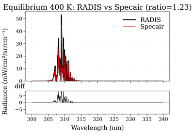
Compare OH(A-X) electronic spectra: RADIS vs Specair
Compare OH(A-X) electronic spectra: RADIS vs Specair
- argmax(value_only=False)[source]
Return wave position of maximum of the Spectrum
Equivalent to the following use of the function
max():s.max(value_only=value_only, return_wmax=True)[1]
See also
- argmin(value_only=False)[source]
Return wave position of minimum of the Spectrum
Equivalent to the following use of the function
min():s.min(value_only=value_only, return_wmin=True)[1]
See also
- cite(format='bibentry')[source]
Prints bibliographic references used to compute this spectrum, as stored in the
referencesdictionary. Default references known to RADIS are listed inradis.db.references.doi.- Parameters:
format (default
'bibentry'. See more inhabanero.content_negotiation())
Examples
from radis import calc_spectrum
s = calc_spectrum(
    1900,
    2300,  # cm-1
    molecule="CO",
    isotope="1,2,3",
    pressure=1.01325,  # bar
    Tvib=2000,  #
    Trot=300,
    mole_fraction=0.1,
    path_length=1,  # cm
    databank="hitran",
)
s.cite()
Returns :
Used for algorithm
------------------
@article{van_den_Bekerom_2021,
    doi = {10.1016/j.jqsrt.2020.107476},
    url = {https://doi.org/10.1016%2Fj.jqsrt.2020.107476},
    year = 2021,
    month = {mar},
    publisher = {Elsevier {BV}},
    volume = {261},
    pages = {107476},
    author = {D.C.M. van den Bekerom and E. Pannier},
    title = {A discrete integral transform for rapid spectral synthesis},
    journal = {Journal of Quantitative Spectroscopy and Radiative Transfer}
}

Used for calculation, rovibrational energies
--------------------------------------------
@article{Pannier_2019,
    doi = {10.1016/j.jqsrt.2018.09.027},
    url = {https://doi.org/10.1016%2Fj.jqsrt.2018.09.027},
    year = 2019,
    month = {jan},
    publisher = {Elsevier {BV}},
    volume = {222-223},
    pages = {12--25},
    author = {Erwan Pannier and Christophe O. Laux},
    title = {{RADIS}: A nonequilibrium line-by-line radiative code for {CO}2 and {HITRAN}-like database species},
    journal = {Journal of Quantitative Spectroscopy and Radiative Transfer}
}

Used for data retrieval
-----------------------
@article{Ginsburg_2019,
    doi = {10.3847/1538-3881/aafc33},
    url = {https://doi.org/10.3847%2F1538-3881%2Faafc33},
    year = 2019,
    month = {feb},
    publisher = {American Astronomical Society},
    volume = {157},
    number = {3},
    pages = {98},
    author = {Adam Ginsburg and Brigitta M. Sip{\H{o}}cz and C. E. Brasseur and Philip S. Cowperthwaite and Matthew W. Craig and Christoph Deil and James Guillochon and Giannina Guzman and Simon Liedtke and Pey Lian Lim and Kelly E. Lockhart and Michael Mommert and Brett M. Morris and Henrik Norman and Madhura Parikh and Magnus V. Persson and Thomas P. Robitaille and Juan-Carlos Segovia and Leo P. Singer and Erik J. Tollerud and Miguel de Val-Borro and Ivan Valtchanov and Julien Woillez and},
    title = {astroquery: An Astronomical Web-querying Package in Python},
    journal = {The Astronomical Journal}
}

Used for line database
----------------------
@article{Gordon_2017,
    doi = {10.1016/j.jqsrt.2017.06.038},
    url = {https://doi.org/10.1016%2Fj.jqsrt.2017.06.038},
    year = 2017,
    month = {dec},
    publisher = {Elsevier {BV}},
    volume = {203},
    pages = {3--69},
    author = {I.E. Gordon and L.S. Rothman and C. Hill and R.V. Kochanov and Y. Tan and P.F. Bernath and M. Birk and V. Boudon and A. Campargue and K.V. Chance and B.J. Drouin and J.-M. Flaud and R.R. Gamache and J.T. Hodges and D. Jacquemart and V.I. Perevalov and A. Perrin and K.P. Shine and M.-A.H. Smith and J. Tennyson and G.C. Toon and H. Tran and V.G. Tyuterev and A. Barbe and A.G. Cs{\'{a}}sz{\'{a}}r and V.M. Devi and T. Furtenbacher and J.J. Harrison and J.-M. Hartmann and A. Jolly and T.J. Johnson and T. Karman and I. Kleiner and A.A. Kyuberis and J. Loos and O.M. Lyulin and S.T. Massie and S.N. Mikhailenko and N. Moazzen-Ahmadi and H.S.P. Müller and O.V. Naumenko and A.V. Nikitin and O.L. Polyansky and M. Rey and M. Rotger and S.W. Sharpe and K. Sung and E. Starikova and S.A. Tashkun and J. Vander Auwera and G. Wagner and J. Wilzewski and P. Wcis{\l}o and S. Yu and E.J. Zak},
    title = {The {HITRAN}2016 molecular spectroscopic database},
    journal = {Journal of Quantitative Spectroscopy and Radiative Transfer}
}

Used for partition function
---------------------------
@article{Gamache_2021,
    doi = {10.1016/j.jqsrt.2021.107713},
    url = {https://doi.org/10.1016%2Fj.jqsrt.2021.107713},
    year = 2021,
    month = {sep},
    publisher = {Elsevier {BV}},
    volume = {271},
    pages = {107713},
    author = {Robert R. Gamache and Bastien Vispoel and Michaël Rey and Andrei Nikitin and Vladimir Tyuterev and Oleg Egorov and Iouli E. Gordon and Vincent Boudon},
    title = {Total internal partition sums for the {HITRAN}2020 database},
    journal = {Journal of Quantitative Spectroscopy and Radiative Transfer}
}
@article{Kochanov_2016,
    doi = {10.1016/j.jqsrt.2016.03.005},
    url = {https://doi.org/10.1016%2Fj.jqsrt.2016.03.005},
    year = 2016,
    month = {jul},
    publisher = {Elsevier {BV}},
    volume = {177},
    pages = {15--30},
    author = {R.V. Kochanov and I.E. Gordon and L.S. Rothman and P. Wcis{\l}o and C. Hill and J.S. Wilzewski},
    title = {{HITRAN} Application Programming Interface ({HAPI}): A comprehensive approach to working with spectroscopic data},
    journal = {Journal of Quantitative Spectroscopy and Radiative Transfer}
}

Used for spectroscopic constants
--------------------------------
@article{Guelachvili_1983,
    doi = {10.1016/0022-2852(83)90203-5},
    url = {https://doi.org/10.1016%2F0022-2852%2883%2990203-5},
    year = 1983,
    month = {mar},
    publisher = {Elsevier {BV}},
    volume = {98},
    number = {1},
    pages = {64--79},
    author = {G. Guelachvili and D. de Villeneuve and R. Farrenq and W. Urban and J. Verges},
    title = {Dunham coefficients for seven isotopic species of {CO}},
    journal = {Journal of Molecular Spectroscopy}
}
Other Examples
See also
- compare_with(other, spectra_only=False, plot=True, wunit='default', verbose=True, rtol=1e-05, ignore_nan=False, ignore_outliers=False, normalize=False, **kwargs)[source]
Compare Spectrum with another Spectrum object.
- Parameters:
other (type Spectrum) – another Spectrum to compare with
spectra_only (boolean, or str) – if
True, only compares spectral quantities (in the same waveunit) and not lines or conditions. If str, compare a particular quantity name. If False, compare everything (including lines and conditions and populations). DefaultFalseplot (boolean) – if
True, use plot_diff to plot all quantities for the 2 spectra and the difference between them. DefaultTrue.wunit (
"nm","cm-1","default") – in which wavespace to compare (and plot). If"default", natural wavespace of first Spectrum is taken.rtol (float) – relative difference to use for spectral quantities comparison
ignore_nan (boolean) – if
True, nans are ignored when comparing spectral quantitiesignore_outliers (boolean, or float) –
if not False, outliers are discarded. i.e, output is determined by:
out = (~np.isclose(I, Ie, rtol=rtol, atol=0)).sum()/len(I) < ignore_outliers
normalize (bool) – Normalize the spectra to be plotted
- Other Parameters:
kwargs (dict) – arguments are forwarded to
plot_diff()- Returns:
equals – return True if spectra are equal (respective to tolerance defined by rtol and other input conditions)
- Return type:
boolean
Examples
Compare two Spectrum objects, or specifically the transmittance:
s1.compare_with(s2)
s1.compare_with(s2, 'transmittance')
Note that you can also simply use
s1 == s2, that usescompare_with()internally:s1 == s2 # will return True or False
See also
- conditions[source]
computation conditions, or experimental parameters, or any metadata you need to store with the Spectrum object.
- Type:
dict
- copy(copy_lines=True, quantity='all', copy_arrays=True)[source]
Returns a copy of this Spectrum object (performs a smart deepcopy)
- Parameters:
copy_lines (bool) – default
Truequantity (‘all’, or one of ‘radiance_noslit’, ‘absorbance’, etc.) – if not ‘all’, copy only one quantity. Default
'all'copy_arrays (bool) – if
False, returned array’s quantity is a pointer to the original Spectrum. Faster, but warning, changing them will then change the original Spectrum. DefaultTrue
Examples
- crop(wmin=None, wmax=None, wunit='default', inplace=True)[source]
Crop spectrum to
wmin-wmaxrange inwunit(inplace)- Parameters:
wmin, wmax (float, or None) – boundaries of spectral range (in
wunit)wunit (
'nm','cm-1','nm_vac') – which waveunit to use forwmin, wmax. Ifdefault: use the default Spectrum wavespace defined withget_waveunit().
- Other Parameters:
inplace (bool) – if
True, modifies the Spectrum object directly. Else, returns a copy. DefaultTrue.- Returns:
s – Cropped Spectrum. If
inplace=True, Spectrum has been updated directly anyway. Allows chaining- Return type:
Examples
Crop to experimental Spectrum, and compare:
from radis import calc_spectrum, load_spec, plot_diff
s = calc_spectrum(...)
s_exp = load_spec('typical_result.spec')
s.crop(s_exp.get_wavelength.min(), s_exp.get_wavelength.max(), 'nm')
plot_diff(s_exp, s)
See also
- fit_model(model, plot=False, confidence=0.9545, verbose=False, debug=False)[source]
Fit a lineshape model to the spectrum.
The model can be a simple lineshape model among
Gaussian1D,Lorentz1D,Voigt1D,or a combination of multiple models.
- Parameters:
model (astropy.modeling.Model or a list of models) – model to fit to the spectrum. If a list is given, a sum of models is fitted
plot (bool) – if True, plot the difference between the model and the spectrum
- Other Parameters:
confidence (0.6827, 0.9545, or 0.9973) – confidence interval to use.
- Returns:
g_fit – the fitted model
y_err – uncertainty on the fitted parameters calculated as the square root of the diagonal of the covariance matrix
Examples
from astropy.modeling import models
s = radis.spectrum_test().crop(2201.7, 2205.1)
g_fit, y_err = s.fit_model(models.Lorentz1D(), plot=True)
Example with 6 Voigt lines:
from astropy.modeling import models
s = radis.spectrum_test().crop(2201.7, 2225.1)
g_fit_list, y_err = s.fit_model([models.Voigt1D() for _ in range(6)], plot=True)
Other Examples
- classmethod from_array(w, I, quantity, wunit=None, Iunit=None, waveunit=None, unit=None, *args, **kwargs)[source]
Construct Spectrum from 2 arrays.
- Parameters:
w, I (array) – waverange and vector
quantity (str) – spectral quantity name
wunit (
'nm','cm-1','nm_vac') – unit of waverange: wavelength in air ('nm'or'nm_air'), wavenumber ('cm-1'), or wavelength in vacuum ('nm_vac'). IfNone, thenwmust be a dimensioned array.Iunit (str) – spectral quantity unit (arbitrary). Ex:
'mW/cm2/sr/nm'for radiance_noslit IfNone, thenImust be a dimensioned array.*args, **kwargs – see
Spectrumdoc
- Other Parameters:
conditions (dict) – physical conditions and calculation parameters
cond_units (dict) – units for conditions
populations (dict) – a dictionary of all species, and levels. Should be compatible with other radiative codes such as Specair output. Suggested format: {molecules: {isotopes: {elec state: rovib levels}}} e.g:
{'CO2':{1: 'X': df}} # with df a Pandas Dataframe
lines (pandas Dataframe) – all lines in databank (necessary for using
line_survey()). Warning if you want to play with the lines content: The signification of columns inlinesmay be specific to a database format. Plus, some additional columns may have been added by the calculation (e.g:EiandSfor emission integral and linestrength in SpectrumFactory). Refer to the code to know what they mean (and their units)
- Returns:
creates a
Spectrumobject- Return type:
Examples
Create a spectrum:
from radis import Spectrum
s = Spectrum.from_array(w, I, 'radiance_noslit',
                       wunit='nm', unit='mW/cm2/sr/nm')
Dimensioned arrays can also be used directly
import astropy.units as u
w = np.linspace(200, 300) * u.nm
I = np.random.rand(len(w)) * u.mW/u.cm**2/u.sr/u.nm
s = Spectrum.from_array(w, I, 'radiance_noslit')
To create a spectrum with absorption and emission components (e.g:
radiance_noslitandtransmittance_noslit, oremisscoeffandabscoeff) call theSpectrumclass directly. Ex:from radis import Spectrum s = Spectrum({'abscoeff': (w, A), 'emisscoeff': (w, E)}, units={'abscoeff': 'cm-1', 'emisscoeff':'W/cm2/sr/nm'}, wunit='nm')
- classmethod from_hdf5(file, wmin=None, wmax=None, wunit=None, columns=None, engine='pytables')[source]
Generates a Spectrum from an HDF5 file. Uses
hdf2spec()- Other Parameters:
wmin, wmax (float) – range of wmin, wmax to load , using
wunit(if None, load everything)columns (list of str) – spectral arrays to load (if None, load everything)
Examples
Spectrum.from_hdf5("rad_hdf.h5", wmin=2100, wmax=2200, columns=['abscoeff', 'emisscoeff'])
See also
- classmethod from_mat(file, quantity, wunit, unit, data_key=None, w_name='nu', I_name=None, index=None, *args, **kwargs)[source]
Construct Spectrum from Matlab
.matfile.- Parameters:
file (str) – file name
quantity (str) – spectral quantity name
wunit (
'nm','cm-1','nm_vac') – unit of waverange: wavelength in air ('nm'), wavenumber ('cm-1'), or wavelength in vacuum ('nm_vac').unit (str) – spectral quantity unit
index (int) – index within Matlab
.matarray.data_key (str) – data key to use within Matlab
.matarray. IfNone, guess.w_name, I_name (str) – key to use to parse the
data[data_key]array and return waverange and quantity.*args, **kwargs – the following inputs are forwarded to
loadmat():'simplify_cells','skiprows'The rest if forwarded to Spectrum and will be registered as a Spectrum condition. seeSpectrumdoc
- Returns:
s – creates a
Spectrumobject- Return type:
Examples
Notes
Internally, the scipy
loadmat()function is used and corresponds todata = scipy.io.loadmat(file, **kwloadmat) data = data[data_key] w, I = data[w_name], data[I_name]
Special keywords can be given to
kwloadmat. See docs ofkwargs.See also
- classmethod from_spec(file)[source]
Generates a Spectrum from a .spec [json] file. Uses
load_spec()
- classmethod from_specutils(spectrum, var='radiance')[source]
Convert a
specutilsSpectrum1Dto aradisSpectrumobject.- Parameters:
spectrum (a
specutilsspecutils.spectra.spectrum1d.Spectrum1D)var (str) – spectral array, default
"radiance"
Examples
Taken from the Specutils website (https://specutils.readthedocs.io/en/stable/#getting-started-with-specutils)
from astropy.io import fits
from astropy import units as u
from specutils import Spectrum1D

f = fits.open('https://data.sdss.org/sas/dr16/sdss/spectro/redux/26/spectra/1323/spec-1323-52797-0012.fits')
# The spectrum is in the second HDU of this file.
specdata = f[1].data

lamb = 10**specdata['loglam'] * u.AA
flux = specdata['flux'] * 10**-17 * u.Unit('erg cm-2 s-1 AA-1')
spec = Spectrum1D(spectral_axis=lamb, flux=flux)

from radis import Spectrum
s = Spectrum.from_specutils(spec)
s.plot(wunit='nm')
See also
- classmethod from_txt(file, quantity, wunit, unit, waveunit=None, *args, **kwargs)[source]
Construct Spectrum from txt file.
- Parameters:
file (str) – file name
quantity (str) – spectral quantity name
wunit (
'nm','cm-1','nm_vac') – unit of waverange: wavelength in air ('nm'), wavenumber ('cm-1'), or wavelength in vacuum ('nm_vac').unit (str) – spectral quantity unit
*args, **kwargs – the following inputs are forwarded to loadtxt:
'delimiter','skiprows'The rest if forwarded to Spectrum. seeSpectrumdoc
- Other Parameters:
delimiter (
',', etc.) – seenumpy.loadtxt()skiprows (int) – see
numpy.loadtxt()argsort (bool) – sorts the arrays in
fileby wavespace. Convenient way to load a file where points have been manually added at the end. DefaultFalse.conditions (dict) – physical conditions and calculation parameters
cond_units (dict) – units for conditions
populations (dict) – a dictionary of all species, and levels. Should be compatible with other radiative codes such as Specair output. Suggested format: {molecules: {isotopes: {elec state: rovib levels}}} e.g:
{'CO2':{1: 'X': df}} # with df a Pandas Dataframe
lines (pandas Dataframe) – all lines in databank (necessary for using
line_survey()). Warning if you want to play with the lines content: The signification of columns inlinesmay be specific to a database format. Plus, some additional columns may have been added by the calculation (e.g:EiandSfor emission integral and linestrength in SpectrumFactory). Refer to the code to know what they mean (and their units)
- Returns:
s – creates a
Spectrumobject- Return type:
Examples
Generate an experimental spectrum from txt. In that example the
delimiterkey is forwarded toloadtxt():from radis import Spectrum s = Spectrum.from_txt('spectrum.csv', 'radiance', wunit='nm', unit='W/cm2/sr/nm', delimiter=',')
To create a spectrum with absorption and emission components (e.g:
radiance_noslitandtransmittance_noslit, oremisscoeffandabscoeff) call theSpectrumclass directly. Ex:from radis import Spectrum s = Spectrum({'abscoeff': (w, A), 'emisscoeff': (w, E)}, units={'abscoeff': 'cm-1', 'emisscoeff':'W/cm2/sr/nm'}, wunit='nm')
Notes
Internally, the numpy
loadtxt()function is used and transposed:w, I = np.loadtxt(file).T
You can use
'delimiter'and ‘skiprows'as arguments.
- classmethod from_xsc(file, conditions={})[source]
Generates a Spectrum from a manually downloaded HITRAN cross-section file under
xscformat. Useshitranxsc()- Parameters:
file (str) – file name
conditions (dictionary) – Conditions metadata added to the Spectrum object. see
Spectrumdoc. Note thatTgasandpressureare automatically read from the cross-section file.
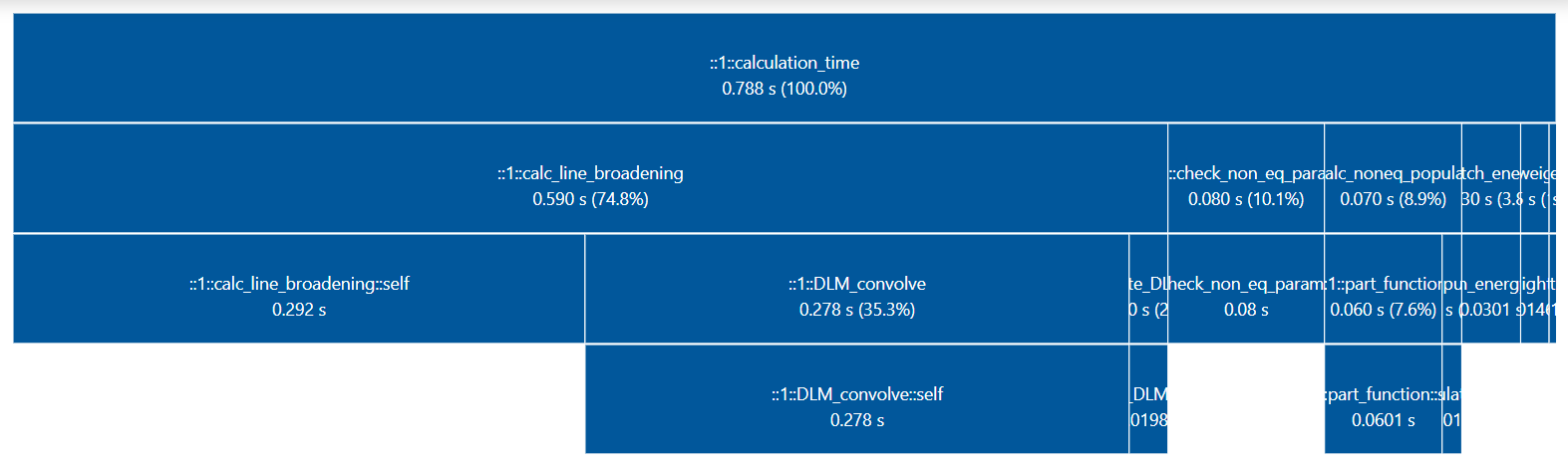
- generate_perf_profile()[source]
Generate a visual/interactive performance profile diagram using
tunaNote
requires a profiler attached to
Spectrum.profilerWarning
deprecated in favor of
print_perf_profile()Examples
s = calc_spectrum(...)
s.generate_perf_profile()
See typical output in https://github.com/radis/radis/pull/325
Note
You can also profile with
tunadirectly:python -m cProfile -o program.prof your_radis_script.py tuna your_radis_script.py
See also
- get(var: ['abscoeff', 'absorbance', 'emissivity_noslit', 'transmittance_noslit', 'radiance_noslit'], wunit='default', Iunit='default', copy=True, trim_nan=False, return_units=False)[source]
Retrieve a spectral quantity from a Spectrum object. You can select wavespace unit, intensity unit, or propagation medium.
- Parameters:
var (variable (
'absorbance','transmittance','xsection'etc.)) – Should be a defined quantity amongCONVOLUTED_QUANTITIESorNON_CONVOLUTED_QUANTITIES. To get the full list of spectral arrays defined in this Spectrum object use theget_vars()method.wunit (
'nm','cm','nm_vac'.) – wavespace unit: wavelength in air ('nm'), wavenumber ('cm-1'), or wavelength in vacuum ('nm_vac'). if"default", default unit for waveunit is used. Seeget_waveunit().Iunit (unit for variable
var) – if"default", default unit for quantityvaris used. See theunitsattribute. Forvar="radiance", one can use per wavelength (~ ‘W/m2/sr/nm’) or per wavenumber (~ ‘W/m2/sr/cm-1’) unitsNote
if using
default, the returned unit may be different from Spectrum.units[var]. e.g, for a Spectrum with radiance stored in ‘mW/cm2/sr/nm’, getting it withwunit='cm-1', Iunit='default'will return Iunit in ‘mW/cm2/sr/cm-1’ for consistency. Usereturn_unitsto be sure about which units are used.
- Other Parameters:
copy (bool) – if
True, returns a copy of the stored quantity (modifying it wont change the Spectrum object). DefaultTrue.trim_nan (bool) – if
True, removesnanon the sides of the spectral array (and corresponding wavespace). DefaultFalse.return_units (bool) – if
True, return dimensioned Astropy arrays. Is usingreturn_units = 'as_str', returnwunitandIunitas extra variables, i.e,w, I, wunit, Iunit = s.get(..., return_units='as_str')DefaultFalse
- Returns:
w, I – wavespace, quantity (ex: wavelength, radiance_noslit). For numpy users, note that these are copies (values) of the Spectrum quantity and not a view (reference): if you modify them the Spectrum is not changed
- Return type:
array-like
Examples
Get transmittance in cm-1:
w, I = s.get('transmittance_noslit', wunit='cm-1')
Get radiance (in wavelength in air):
_, R = s.get('radiance_noslit', wunit='nm', Iunit='W/cm2/sr/nm')
Use with
return_unitsto get dimensioned Astropy Quantitiesw, R = s.get('radiance_noslit', return_units=True)
See also
- get_baseline(algorithm='als', **kwargs)[source]
Calculate and returns a baseline
- Parameters:
s (Spectrum) – Spectrum which needs a baseline
var (str) – on which spectral quantity to read the baseline. Default
'radiance'. SeeSPECTRAL_QUANTITIESalgorithm (‘als’, ‘polynomial’) – Asymmetric least square or Polynomial fit
**kwargs (dict) – additional parameters to send to the algorithm. By default, for ‘polynomial’:
for ‘als’:
- **kwargs = {“asymmetry_param”: 0.05,
“smoothness_param”: 1e6}
- Returns:
baseline – Spectrum object where intensity is the baseline of s
- Return type:
Examples
See also
- get_condition(condition, unit='default', return_unit=False)[source]
Get condition in arbitrary unit
If condition was stored as a dimensioned value, return a dimensioend value (converted to the right unit) If condition was stored as a non dimensioned value, return a non dimensioned value (still converted to the right unit)
- Parameters:
condition (str) – condition name
unit (str) – unit name
return_unit (bool) – if True, return value and unit separately (value is not dimensioned in this case)
Examples
Get pressure (as float, non dimensioned) in Pascal:
s = radis.spectrum_test()
pressure_Pa, _ = s.get_condition("pressure", "Pa", return_unit=True)
Get pressure and convert it to a dimensioned value:
from radis.phys.units import Unit as u
s = radis.spectrum_test()
pressure_value, pressure_unit = s.get_condition("pressure", return_unit=True)
pressure = pressure_value * u(pressure_unit)
- get_integral(var, wunit='default', Iunit='default', **kwargs)[source]
Returns integral of variable ‘var’ over waverange.
- Parameters:
var (str) – spectral quantity to integrate
wunit (str) – over which waverange to integrated. If
default, use the default Spectrum wavespace defined withget_waveunit().Iunit (str) – default
'default'Warning
this is the unit of the quantity, not the unit of the integral. Don’t forget to multiply by
wunit
- Other Parameters:
- Returns:
integral – integral in [Iunit]*[wunit]
- Return type:
float
See also
- get_name()[source]
Return Spectrum name.
If not defined, returns either the
filename if Spectrum was loaded from a file, or the'spectrum{id}'with the Pythonidobject
- get_populations(molecule=None, isotope=None, electronic_state=None, show_warning=True)[source]
Return populations that are featured in the spectrum, either as upper or lower levels.
- Parameters:
molecule (str, or None) – if None, only one molecule must be defined. Else, an error is raised
isotope (int, or None) – isotope number. if None, only one isotope must be defined. Else, an error is raised
electronic_state (str) – if None, only one electronic state must be defined. Else, an error is raised
show_warning (bool) – if False, turns off warning about meaning of populations, see Notes and discussion on https://github.com/radis/radis/issues/508.
- Returns:
pandas dataframe of levels, where levels are the index,
and ‘Evib’ and ‘nvib’ are featured
Notes
Structure:
{molecule: {isotope: {electronic_state: {'vib': pandas Dataframe,    # (copy of) vib levels
                                         'rovib': pandas Dataframe,  # (copy of) rovib levels
                                         'Ia': float    # isotopic abundance
                                         }}}}
(If Spectrum generated with RADIS, structure should match that of SpectrumFactory.get_populations())
Examples
An example on how different are populations used for partition function and spectrum calculations
#%% CO2 example
# For instance, plot populations of a given vibrational level, v1,v2,v3=(0,1,0)
import radis
s = radis.spectrum_test(molecule="CO2", Tvib=3000, Trot=1000,
                        export_lines=True,
                        export_populations="rovib",
                        isotope=1)
pops = s.get_populations("CO2")["rovib"]

import matplotlib.pyplot as plt
pops.query("v1==0 & v2==1 & v3==0").plot("j", "n",
                                         label="pops. used to compute partition functions")
s.lines.query("v1l==0 & v2l==1 & v3l==0").plot("jl", "nl", ax=plt.gca(), kind="scatter", color="r",
                                               label="pops. of visible absorbing lines")
plt.legend()
plt.xlim((0,70))
See also
- get_power(unit='mW/cm2/sr')[source]
Returns integrated radiance (no slit) power density.
- Parameters:
Iunit (str) – power unit.
- Returns:
P – radiated power in
unit- Return type:
float
Examples
s.get_power('W/cm2/sr')
See also
- get_quantities()[source]
Returns all spectral quantities stored in this object (convoluted or non convoluted). Wrapper to
get_vars()
- get_radiance(Iunit='mW/cm2/sr/nm', copy=True)[source]
Return radiance in whatever unit, and can even convert from ~1/nm to ~1/cm-1 (and the other way round)
- Other Parameters:
copy (boolean) – if
True, returns a copy of the stored waverange (modifying it wont change the Spectrum object). DefaultTrue.
See also
- get_radiance_noslit(Iunit='mW/cm2/sr/nm', copy=True)[source]
Return radiance (non convoluted) in whatever unit, and can even convert from ~1/nm to ~1/cm-1 (and the other way round)
- Other Parameters:
copy (boolean) – if
True, returns a copy of the stored waverange (modifying it wont change the Spectrum object). DefaultTrue.
See also
- get_rovib_levels(molecule=None, isotope=None, electronic_state=None, first=None)[source]
Return rovibrational levels calculated in the spectrum (energies, populations)
- Parameters:
molecule (str, or None) – if None, only one molecule must be defined. Else, an error is raised
isotope (int, or None) – isotope number. if None, only one isotope must be defined. Else, an error is raised
electronic_state (str) – if None, only one electronic state must be defined. Else, an error is raised
first (int, or ‘all’ or None) – only show the first N levels. If None or ‘all’, all levels are shown
- Returns:
out – pandas dataframe of levels, where levels are the index, and ‘Evib’ and ‘nvib’ are featured
- Return type:
pandas DataFrame
- get_slit(wunit='same')[source]
Get slit function that was applied to the Spectrum.
- Returns:
wslit, Islit – slit function with wslit in Spectrum
waveunit. Seeget_waveunit()- Return type:
array
- get_vars()[source]
Returns all spectral quantities stored in this object (convoluted or non convoluted)
- get_vib_levels(molecule=None, isotope=None, electronic_state=None, first=None)[source]
Return vibrational levels in the spectrum (energies, populations)
- Parameters:
molecule (str, or None) – if None, only one molecule must be defined. Else, an error is raised
isotope (int, or None) – isotope number. if None, only one isotope must be defined. Else, an error is raised
electronic_state (str) – if None, only one electronic state must be defined. Else, an error is raised
first (int, or ‘all’ or None) – only show the first N levels. If None or ‘all’, all levels are shown
- Returns:
out – pandas dataframe of levels, where levels are the index, and ‘Evib’ and ‘nvib’ are featured
- Return type:
pandas DataFrame
- get_wavelength(medium='air', copy=True)[source]
Return wavelength in defined medium.
- Parameters:
medium (
'air','vacuum') – returns wavelength as seen in air, or vacuum. Default'air'. Seevacuum2air(),air2vacuum()- Other Parameters:
copy (boolean) – if
True, returns a copy of the stored waverange (modifying it wont change the Spectrum object). DefaultTrue.- Returns:
w – (a copy of) spectrum wavelength for convoluted or non convoluted quantities
- Return type:
array_like
See also
- get_wavenumber(copy=True)[source]
Return wavenumber (if the same for all quantities)
- Other Parameters:
copy (boolean) – if
True, returns a copy of the stored waverange (modifying it wont change the Spectrum object). DefaultTrue.- Returns:
w – (a copy of) spectrum wavenumber for convoluted or non convoluted quantities
- Return type:
array_like
- get_waveunit()[source]
Returns whether this spectrum is defined in wavelength (nm) or wavenumber (cm-1)
- has_nan(ignore_wavespace=True) bool[source]
- Parameters:
s (Spectrum) – radis Spectrum.
- Returns:
b – returns whether Spectrum has
nan- Return type:
bool
- is_at_equilibrium(check='warn', verbose=False)[source]
Returns whether this spectrum is at (thermal) equilibrium. Reads the
thermal_equilibriumkey in Spectrum conditions. It does not imply chemical equilibrium (mole fractions are still arbitrary)If they are defined, also check that the following assertions are True:
Tvib = Trot = Tgas self_absorption = True overpopulation = None
If they are not, still trust the value in Spectrum conditions, but raise a warning.
- Other Parameters:
check (
'warn','error','ignore') – what to do if Spectrum conditions dont match the given equilibrium state: raise a warning, raise an error, or just ignore and dont even check. Default'warn'.verbose (bool) – if
True, print why is the spectrum is not at equilibrium, if applicable.
- is_optically_thin()[source]
Returns whether the spectrum is optically thin, based on the value on the self_absorption key in conditions.
If not given, raises an error
- line_survey(overlay=None, wunit='cm-1', Iunit='hitran', medium='air', cutoff=None, plot='S', lineinfo=['int', 'A', 'El'], barwidth='hwhm_voigt', yscale='log', writefile=None, *args, **kwargs)[source]
Plot line survey (all linestrengths used for calculation).
Output in Plotly (HTML).
- Parameters:
overlay (tuple (w, I, [name], [units]), or list of tuples) – Plot
(w, I)on a secondary axis. Useful to compare linestrength with calculated / measured data:LineSurvey(overlay='abscoeff')
wunit (
'nm','cm-1') – Wavelength / wavenumber units.Iunit (
'hitran','splot') – Linestrength output units:'hitran': (cm-1/(molecule/cm-2))'splot': (cm-1/atm) (Spectraplot units [2]_)
Note: if not
None, the cutoff criteria is applied in this unit. Not used ifplotis not'S'.medium (
'air','vacuum') – Show wavelength either in air or vacuum. Default'air'.plot (str) – What to plot. Default
'S'(scaled linestrength), but it can be any key in the lines, such as population ('nu') or Einstein coefficient ('A').lineinfo (list, or
'all') – Extra line information to plot. Should be a column name in the databank (s.lines). For instance:'int','selbrd', etc. Default is ['int','A','El'].
- Other Parameters:
writefile (str) – If not
None, a valid filename to save the plot in.htmlformat. IfNone, use the returnedfigobject to display the plot.yscale (
'log','linear') – Default'log'.barwidth (float or str) – If float, width of bars in
wunitas a fraction of full range, i.e.:barwidth=0.01
Makes bars span 1% of the full range. If
str, uses the column as width. Example:barwidth = 'hwhm_voigt'
- Returns:
fig (plotly.graph_objects.Figure) – If using a Jupyter notebook, the plot will appear. Otherwise, use
writefileto export to an HTML file.Plot in Plotly.
Examples
An example using the
SpectrumFactoryto generate a spectrum:from radis import SpectrumFactory sf = SpectrumFactory( wavenum_min=2380, wavenum_max=2400, mole_fraction=400e-6, path_length=100, # cm isotope=[1], export_lines=True, # required for LineSurvey! db_use_cached=True, ) sf.load_databank("HITRAN-CO2-TEST") s = sf.eq_spectrum(Tgas=1500) s.apply_slit(0.5) s.line_survey( overlay="radiance_noslit", barwidth=0.01, lineinfo="all" ) # or barwidth='hwhm_voigt'
See the output in [1]_.
References
See also
- lines[source]
informations on emitting or absorbing lines that contribute to the spectrum.
See also
line_survey()
- max(value_only=False, return_wmax=False)[source]
Maximum of the Spectrum, if only one spectral quantity is available:
s.max()
Returns a dimensioned quantity by default, with the default unit of the spectrum. If
value_only=False, a float is returned, without dimensions.If there are multiple arrays in your Spectrum, use
take(), e.g.s.take('radiance').max()
- Parameters:
value_only (bool)
return_position (bool) – if True, returns wavelength or wavenumber of maximum, in the Spectrum unit.
Examples
Normalize a spectrum (we could also have used
normalize()directly)s /= s.max()
Below is a slightly more advanced use case, convenient to process non-calibrated experimental data.
Imagine we want to remove a baseline that we have identified to originate from a particular species, modelled by spectrum
s, but whose intensity (and units) are not the same as that of the experimental spectrum.We substract exactly the intensity that correspond to the intensity on a given range
w1, w2of the experimental spectrums_exp, using a combination oftake(),normalize(),crop()andmax():s_exp -= s.take('radiance').normalize() * s_exp.crop((w1, w2)), inplace=False).max()
Other Examples
Get max position
wmaxs = radis.spectrum_test() max, wmax = s.max(return_wmax=True)
Note that the later can also be achieved with
argmax()wmax = s.argmax()
Example #7: Database fitting using SpecDatabase.fit_spectrum
Example #7: Database fitting using SpecDatabase.fit_spectrumSee also
- min(value_only=True, return_wmin=False)[source]
Minimum of the Spectrum, if only one spectral quantity is available
s.min()
Returns a dimensioned quantity by default, with the default unit of the spectrum. If
value_only=False, a float is returned, without dimensions.If there are multiple arrays in your Spectrum, use
take(), e.g.s.take('radiance').min()
Other Examples
Get min position
wmins = radis.spectrum_test() min, wmin = s.min(return_wmin=True)
Note that the later can also be achieved with
argmin()wmax = s.argmin()
See also
- normalize(normalize_how='max', wrange=(), wunit=None, inplace=False, force=False, verbose=False, return_norm=False)[source]
Normalise the Spectrum, if only one spectral quantity is available.
- Parameters:
normalize_how (
'max','area','mean') – how to normalize.'max'is the default but may not be suited for very noisy experimental spectra.'area'will normalize the integral to 1.'mean'will normalize by the mean amplitude valuewrange (tuple of floats, float) – normalize on this range if a tuple, else normalise at that point. If an empty tuple, use the entire range.
wunit (
"nm","cm-1","nm_vac") – unit of the normalisation range above. IfNone, use the spectrum default waveunit.inplace (bool) – if
True, changes the Spectrum.
- Other Parameters:
force (boolean) – By default, normalizing some parameters such as transmittance is forbidden because considered non-physical. Use force=True if you really want to.
Examples
s.normalize("max", (4200, 4800), inplace=True).plot()
If there are multiple arrays in your Spectrum, use
take(), e.g.s.take('radiance').normalize(wrange=(4200, 4800)).plot()
- offset(offset: Spectrum, unit: float, inplace: str = True) Spectrum[source]
Offset the spectrum by a wavelength or wavenumber (inplace)
- Parameters:
offset (float) – Constant to add to all quantities in the Spectrum.
unit (‘nm’ or ‘cm-1’) – unit for
offset
- Other Parameters:
inplace (bool) – if
True, modifies the Spectrum object directly. Else, returns a copy. DefaultTrue.- Returns:
s – Offset Spectrum. If
inplace=True, Spectrum has been updated directly anyway. Allows chaining.- Return type:
Examples
s.offset(5, 'nm')
- plot(var: ['abscoeff', 'absorbance', 'emissivity_noslit', 'transmittance_noslit', 'radiance_noslit'] = None, wunit='default', Iunit='default', show_points=False, nfig=None, yscale='linear', show_medium='vacuum_only', normalize=False, force=False, plot_by_parts=False, show=True, show_ruler=False, plotting_library='default', **kwargs)[source]
Plot a
Spectrumobject.Note
default plotting library and templates can be edited in
radis.config[“plot”]- Parameters:
var (variable (
absorbance,transmittance,transmittance_noslit,xsection, etc.)) – For full list seeget_vars(). IfNone, plot the first thing in the Spectrum. DefaultNone.wunit (
'default','nm','cm-1','nm_vac',) – wavelength air, wavenumber, or wavelength vacuum. If'default', Spectrumget_waveunit()is used.Iunit (unit for variable) – if
default, default unit for quantityvaris used. for radiance, one can use per wavelength (~W/m2/sr/nm) or per wavenumber (~W/m2/sr/cm-1) units
- Other Parameters:
show_points (boolean) – show calculated points. Default
True.nfig (int, None, or ‘same’) – plot on a particular figure. ‘same’ plots on current figure. For instance:
s1.plot()
s2.plot(nfig='same')
show_medium (bool,
'vacuum_only') – ifTrueandwunitare wavelengths, plot the propagation medium in the xaxis label ([air]or[vacuum]). If'vacuum_only', plot only ifwunit=='nm_vac'. Default'vacuum_only'(prevents from inadvertently plotting spectra with different propagation medium on the same graph).yscale (‘linear’, ‘log’) – plot yscale
normalize (boolean, or tuple.) – option to normalize quantity to 1 (ex: for radiance). Default
Falseplot_by_parts (bool) – if
True, look for discontinuities in the wavespace and plot the different parts without connecting lines. Useful for experimental spectra produced by overlapping step-and-glue. Additional parameters read fromkwargs:split_thresholdandcutwings. See more insplit_and_plot_by_parts().force (bool) – plotting on an existing figure is forbidden if labels are not the same. Use
force=Trueto ignore that.show (bool) – show figure. Default
False. Will still show the figure in interactive mode, e.g,%matplotlib inlinein a Notebook.show_ruler (bool) – if
True, add a ruler tool to the Matplotlib toolbar. Convenient to measure distances between peaks, etc.Warning
still experimental ! Try it, feedback welcome !
plotting_library (str) – Specifies the plotting library to use for rendering the plot. Options:
- “auto” (default): Automatically selects the plotting backend based on the environment.
If running in a Jupyter notebook, it defaults to Plotly for interactive plots.
If running in a standard Python environment, it defaults to Matplotlib for static plots.
“plotly”: Forces the use of Plotly for interactive plots.
“matplotlib”: Forces the use of Matplotlib for static plots.
**kwargs (**dict) – kwargs forwarded as argument to plot (e.g: lineshape attributes:
lw=3, color='r')
- Returns:
line plot
- Return type:
line
Examples
Plot an
experimental_spectrum()in arbitrary units:s = experimental_spectrum(..., Iunit='mW/cm2/sr/nm') s.plot(Iunit='W/cm2/sr/cm-1')
See more examples in the plot Spectral quantities page.
See also
- plot_populations(what=None, nunit='', correct_for_abundance=False, **kwargs)[source]
Plots vib populations if given and format is valid.
- Parameters:
what (‘vib’, ‘rovib’, None) – if None plot everything
nunit (‘’, ‘cm-3’) – plot either in a fraction of vibrational levels, or a molecule number in in cm-3
correct_for_abundance (boolean) – if
True, multiplies each population by the isotopic abundance (as it is done during the calculation of emission integral)kwargs (**dict) – are forwarded to the plot
Examples
See also
- plot_slit(wunit=None, waveunit=None)[source]
Plot slit function that was applied to the Spectrum.
If dispersion was used (see
apply_slit()) the different slits are built again and plotted too (dotted).- Parameters:
wunit (
'nm','cm-1', orNone) – plot slit in wavelength or wavenumber. IfNone, use the unit the slit in which the slit function was given. DefaultNone- Returns:
fix, ax – figure and ax
- Return type:
matplotlib objects
Examples
s = radis.spectrum_test()
s.apply_slit((0.4, 0.6), "nm")  # add trapezoidal slit function
s.plot_slit()   # plot the slit function that was applied
See also
- populations[source]
populations of rovibrational levels used to compute partition functions of the spectrum
See also
get_populations(),plot_populations()
- print_conditions(**kwargs)[source]
Prints all physical / computational parameters.
- Parameters:
kwargs (dict) – refer to
print_conditions()
Examples
s = radis.spectrum_test()
s.print_conditions()
You can also simply print the Spectrum object directly:
s = radis.spectrum_test()
print(s)
Both syntaxes above will return (in radis==0.15):
# output >>

    Spectrum Name:  CO-hitran-700K-#3680
    Spectral Quantities
    ----------------------------------------
       abscoeff     [cm-1]  (40,002 points)
       absorbance   (40,002 points)
       emissivity_noslit    (40,002 points)
       transmittance_noslit         (40,002 points)
       radiance_noslit      [mW/cm2/sr/cm-1]        (40,002 points)
    Physical Conditions
    ----------------------------------------
       Tgas                 700 K
       Trot                 700 K
       Tvib                 700 K
       isotope              1,2,3
       mole_fraction        0.1
       molecule             CO
       overpopulation       None
       path_length          1 cm
       pressure             1.01325 bar
       rot_distribution     boltzmann
       self_absorption      True
       state                X
       thermal_equilibrium  True
       vib_distribution     boltzmann
       wavenum_max          2300.0000 cm-1
       wavenum_min          1900.0000 cm-1
    Computation Parameters
    ----------------------------------------
       NwG                  3
       NwL                  5
       Tref                 296 K
       broadening_method    voigt_poly
       cutoff               1e-27 cm-1/(#.cm-2)
       dbformat             hitran
       dbpath               C:\Users\erwan\.radisdb\hitran\CO.hdf5
       default_output_unit  cm-1
       diluents             {'air': 0.9}
       folding_thresh       1e-06
       include_neighbouring_lines  True
       memory_mapping_engine  auto
       neighbour_lines      0 cm-1
       optimization         simple
       parsum_mode          full summation
       profiler             {'spectrum_calculation': {'check_line_databank': ...
       pseudo_continuum_threshold  0
       radis_version        0.14
       sparse_ldm           True
       spectral_points      40000.0
       truncation           50 cm-1
       waveunit             cm-1
       wstep                0.01 cm-1
       zero_padding         40002
    Config parameters
    ----------------------------------------
       DEFAULT_DOWNLOAD_PATH  ~/.radisdb
       GRIDPOINTS_PER_LINEWIDTH_ERROR_THRESHOLD  1
       GRIDPOINTS_PER_LINEWIDTH_WARN_THRESHOLD  3
       SPARSE_WAVERANGE     auto
    Information
    ----------------------------------------
       calculation_time     0.11549490000000162 s
       chunksize            None
       db_use_cached        True
       dxG                  0.1375350788016573
       dxL                  0.20180288881201608
       export_lines         False
       export_populations   None
       export_rovib_fraction  True
       levelsfmt            None
       lines_calculated     742
       lines_cutoff         0
       lines_in_continuum   0
       load_energies        False
       lvl_use_cached       True
       parfuncpath          None
       total_lines          742
       warning_broadening_threshold  0.01
       warning_linestrength_cutoff  0.01
       wavenum_max_calc     2300.0000 cm-1
       wavenum_min_calc     1900.0000 cm-1
    ----------------------------------------
See also
- print_perf_profile(number_format='{:.3f}', precision=16)[source]
Prints Profiler output dictionary in a structured manner.
Example
Spectrum.print_perf_profile() # output >> spectrum_calculation 0.189s ████████████████ check_line_databank 0.000s check_non_eq_param 0.042s ███ fetch_energy_5 0.015s █ calc_weight_trans 0.008s reinitialize 0.002s copy_database 0.000s memory_usage_warning 0.002s reset_population 0.000s calc_noneq_population 0.041s ███ part_function 0.035s ██ population 0.006s scaled_non_eq_linestrength 0.005s map_part_func 0.001s corrected_population_se 0.003s calc_emission_integral 0.006s applied_linestrength_cutoff 0.002s calc_lineshift 0.001s calc_hwhm 0.007s generate_wavenumber_arrays 0.001s calc_line_broadening 0.074s ██████ precompute_LDM_lineshapes 0.012s LDM_Initialized_vectors 0.000s LDM_closest_matching_line 0.001s LDM_Distribute_lines 0.001s LDM_convolve 0.060s █████ others 0.001s calc_other_spectral_quan 0.003s generate_spectrum_obj 0.000s others -0.016s- Other Parameters:
precision (int, optional) – total number of blocks. Default 16.
See also
- recalc_gpu(var='abscoeff', wunit='default', Iunit='default', pressure=None, Tgas=None, mole_fraction=None, path_length=None, slit_function=None)[source]
Recalculate the spectrum based on new input parameters. Can only be called for spectrum objects produced by
eq_spectrum_gpu(). This method is used internally byeq_spectrum_gpu_interactive(). Parameters may be passed as arguments, or updated directly inconditions, after which spectrum.recalc_gpu() may be called without passing arguments.- Parameters:
var (variable (
absorbance,transmittance,transmittance_noslit,xsection, etc.)) – For full list seeget_vars(). IfNone, plot the first thing in the Spectrum. DefaultNone.wunit (
'nm','cm-1','nm_vac'orNone) – wavelength in air ('nm'), wavenumber ('cm-1'), or wavelength in vacuum ('nm_vac'). IfNone,'wavespace'must be defined inconditions.Iunit (unit for variable) – if
default, default unit for quantityvaris used. for radiance, one can use per wavelength (~W/m2/sr/nm) or per wavenumber (~W/m2/sr/cm-1) unitspressure (float, optional) – Pressure in [bar]
Tgas (float, optional) – Equilibrium temperature in [K]
mole_fraction (float, optional) – Mole fraction
path_length (float, optional) – Absroption length in [cm]
slit_function (float, optional) – Slit FWHM in [cm-1]
- Returns:
new_y – The recalculated array specified by the
varkeyword.- Return type:
numpy.ndarray[np.fltoat32]
Examples
s = sf.eq_spectrum_gpu(
    Tgas=1100.0,  # K
    pressure=1,  # bar
    mole_fraction=0.8,
    path_length=0.2,  # cm
)

I = []
for T in [300.0, 1000.0, 2000.0]:
    I.append(s.recalc_gpu('radiance', Tgas=T)
- resample(w_new, unit='same', out_of_bounds='nan', energy_threshold='default', print_conservation=False, inplace=True, **kwargs)[source]
Resample spectrum over a new wavelength/wavenumber range.
Warning
This may result in information loss. Resampling is done with oversampling and spline interpolation. These parameters can be adjusted, and energy conservation ensured with the appropriate parameters.
To minimize information loss, always resample the high-resolution spectrum over the low-resolution spectrum, i.e.
s_highres.resample(s_lowres)
Fills with
'nan'or transparent medium (transmittance 1, radiance 0) when out of bound (seeout_of_bounds)- Parameters:
w_new (array, or Spectrum) – new wavespace to resample the spectrum on. Must be inclosed in the current wavespace (we won’t extrapolate) One can also give a Spectrum directly:
s1.resample(s2.get_wavenumber())
s1.resample(s2)            # also valid
unit (
'same','nm','cm-1','nm_vac') – unit of new wavespace. It'same'it is assumed to be the current waveunit. Default'same'. The spectrum waveunit is changed to this unit after resampling (i.e: a spectrum calculated and stored incm-1but resampled innmwill be stored innmfrom now on). If'nm', wavelength in air. If'nm_vac', wavelength in vacuum.out_of_bounds (
'transparent','nan','error') – what to do if resampling is out of bounds.'transparent': fills with transparent medium. ‘nan’: fill with nan.'error': raises an error. Default'nan'medium (
'air','vacuum', or'default') – in which medium is the new waverange is calculated if it is given in ‘nm’. Ignored if unit=’cm-1’
- Other Parameters:
energy_threshold (float or
Noneor'default') -- if energy conservation (integrals on the intersecting range) is above this threshold, raise an error. If ``None, dont check for energy conservation. If'default', look up the value inradis.config[“RESAMPLING_TOLERANCE_THRESHOLD”] Default'default'print_conservation (boolean) – if
True, prints energy conservation. DefaultFalse.inplace (boolean) – if
True, modifies the Spectrum object directly. Else, returns a copy. DefaultTrue.**kwargs (**dict) – all other arguments are sent to
radis.misc.signal.resample()
- Returns:
Spectrum – object has been modified anyway.
- Return type:
resampled Spectrum object. If using
inplace=True, the Spectrum
Examples
Convert a Spectrum in wavenumber to wavelengths:
s_nm = s.resample(s.get_wavelength(), "nm", inplace=False)
- resample_even(energy_threshold=0.005, print_conservation=False, inplace=True)[source]
Resample spectrum over the same waverange, but evenly spaced.
Warning
This may result in information loss. Resampling is done with oversampling and spline interpolation. These parameters can be adjusted, and energy conservation ensured with the appropriate parameters.
- Parameters:
energy_threshold (float or
None) – if energy conservation (integrals on the intersecting range) is above this threshold, raise an error. IfNone, dont check for energy conservation Default 5e-3 (0.5%)print_conservation (boolean) – if
True, prints energy conservation. DefaultFalse.inplace (boolean) – if
True, modifies the Spectrum object directly. Else, returns a copy. DefaultTrue.**kwargs (**dict) – all other arguments are sent to
radis.misc.signal.resample()
- Returns:
Spectrum – object has been modified anyway.
- Return type:
resampled Spectrum object. If using
inplace=True, the Spectrum
Examples
- rescale_mole_fraction(new_mole_fraction, old_mole_fraction=None, inplace=True, ignore_warnings=False, force=False, verbose=True)[source]
Update spectrum with new molar fraction Convoluted values (with slit) are dropped in the process.
- Parameters:
new_mole_fraction (float) – new mole fraction
old_mole_fraction (float, or None) – if None, current mole fraction (conditions[‘mole_fraction’]) is used
- Other Parameters:
inplace (boolean) – if
True, modifies the Spectrum object directly. Else, returns a copy. DefaultTrue.force (boolean) – if False, won’t allow rescaling to 0 (not to loose information). Default
False
- Returns:
s – Cropped Spectrum. If
inplace=True, Spectrum has been updated directly anyway. Allows chaining- Return type:
Examples
s.rescale_mole_fraction(0.2)

Calculate and Compare Spectra for Multiple Molecules
Calculate and Compare Spectra for Multiple MoleculesNotes
Implementation:
similar to rescale_path_length() but we have to scale abscoeff & emisscoeff Note that this is valid only for small changes in mole fractions. Then, the change in line broadening becomes significant
See also
- rescale_path_length(new_path_length, old_path_length=None, inplace=True, force=False)[source]
Rescale spectrum to new path length. Starts from absorption coefficient and emission coefficient, and solves the RTE again for the new path length Convoluted values (with slit) are dropped in the process.
- Parameters:
new_path_length (float) – new path length
old_path_length (float, or None) – if None, current path length (conditions[‘path_length’]) is used
- Other Parameters:
inplace (boolean) – if
True, modifies the Spectrum object directly. Else, returns a copy. DefaultTrue.force (boolean) – if False, won’t allow rescaling to 0 (not to loose information). Default
False
- Returns:
s – Cropped Spectrum. If
inplace=True, Spectrum has been updated directly anyway. Allows chaining- Return type:
Examples
for path in [0.1, 10, 100]:
    s.rescale_path_length(10, inplace=False).plot(nfig='same')
Additionally, you can also use astropy units in the input arguments, for example:
# preparing a test spectrum :
import radis
s = radis.spectrum_test()

# rescaling :
import astropy.units as u
s.rescale_path_length(1 * u.km).plot()
Notes
Implementation:
To deal with all the input cases, we first make a list of what has to be recomputed, and what has to be recalculated
See also
- savetxt(filename, var, wunit='default', Iunit='default')[source]
Export spectral quantity var to filename.
- (note that by doing this you will loose additional information, such
as the calculation conditions or the units. You better save a Spectrum object under a .spec file with
store()and load it afterwards withload_spec())
- Parameters:
filename (str) – file name
var (str) – which spectral variable ot export
- Other Parameters:
wunit, Iunit, medium (str) – see
get()for more information
Notes
Export variable as:
np.savetxt(filename, np.vstack(self.get(var, wunit=wunit, Iunit=Iunit,
                                    medium=medium)).T, header=header)
See also
- sort(inplace=True)[source]
Sort the Spectrum by wavelength / wavenumber.
- Parameters:
inplace (bool, optional) – if
True, modifies the Spectrum object directly. The default isTrue.- Returns:
s – sorted Spectrum. If
inplace=True, Spectrum has been updated directly anyway. Allows chaining.- Return type:
Examples
- store(path, discard=['lines', 'populations'], compress=True, add_info=None, add_date=None, if_exists_then='error', verbose=True)[source]
Save a Spectrum object in JSON format. Object can be recovered with
load_spec(). If many Spectrum are saved in a same folder you can view their properties with theSpecDatabasestructure.- Parameters:
path (str or file-like object) – If a string: path to folder (database) or file. If a folder, file is saved to database and name is generated automatically. If a file name, then Spectrum is saved to this file and the later formatting options dont apply.
If a file-like object (e.g.,
io.BytesIO,io.StringIO): writes directly to the object without any file system operations. UseBytesIOwhencompress=True(binary output), useStringIOwhencompress=False(text output). When using file-like objects, theadd_date,add_info, andif_exists_thenparameters are ignored.compress (boolean) – if
False, save under text format, readable with any editor. ifTrue, saves under binary format. Faster and takes less space. If2, removes all quantities that can be regenerated with s.update(), e.g, transmittance if abscoeff and path length are given, radiance if emisscoeff and abscoeff are given in non-optically thin case, etc. DefaultTrue.add_info (list) – append these parameters and their values if they are in conditions example:
add_info = ['Tvib', 'Trot']
discard (list of str) – parameters to exclude, for instance to save some memory for instance Default [
lines,populations]: retrieved Spectrum looses theline_survey()ability, andplot_populations()(but it saves tons of memory!)if_exists_then (
'increment','replace','error','ignore') – what to do if file already exists. If increment an incremental digit is added. If replace file is replaced (yeah). If'ignore'no file is created. If error (or anything else) an error is raised. Defaulterror
- Returns:
If path was a string: filename used (may be different from given path as new info or incremental identifiers are added). If path was a file-like object: returns the same object.
- Return type:
str or file-like object
Notes
If many spectra are stored in a folder, it may be time to set up a
SpecDatabasestructure to easily see all Spectrum conditions and get Spectrum that suits specific parameters.Examples
Store a spectrum in compressed mode, regenerate quantities after loading:
from radis import load_spec
s.store('test.spec', compress=True)   # s is a Spectrum
s2 = load_spec('test.spec')
s2.update()                           # regenerate missing quantities
Store a spectrum to a BytesIO buffer (no disk write):
from io import BytesIO
buffer = BytesIO()
s.store(buffer, compress=True)
buffer.seek(0)  # Reset position for reading
# buffer.getvalue() contains the serialized spectrum
Examples using
radis.spectrum.spectrum.Spectrum.store¶See also
- take(var, copy_lines=False, copy_arrays=True)[source]
- Parameters:
var (str) – spectral quantity (
'absorbance','transmittance','xsection'etc.)- Other Parameters:
copy_lines (bool) – if
True, exports.lines. DefaultFalsecopy_arrays (bool) – if
False, returned array’s quantity is a pointer to the original Spectrum. Faster, but warning, changing them will then change the original Spectrum. DefaultTrue
- Returns:
s – same Spectrum with only the
varspectral quantity- Return type:
Examples
Use
taketo chain other commandss.take('radiance').normalize().plot()
- to_hdf5(file, engine='pytables')[source]
Convert a
radisSpectrumobject to HDF5 format. Usesspec2hdf()- Parameters:
file (str) – path to save the HDF5 file
engine (str, optional) – Which HDF5 library to use for reading/writing data. Options are:
‘pytables’ (default) : Use PyTables library
- Return type:
The spectrum is saved to disk in HDF5 format
Note
The HDF5 file will contain all spectral arrays in an ‘arrays’ group with their units as metadata, the lines database in a ‘lines’ group if present, populations in metadata if present, and conditions and references in metadata.
Use
from_hdf5()to load the spectrum back.Examples
s.to_hdf5('spectrum.h5')
Load back with:
from radis import Spectrum
s2 = Spectrum.from_hdf5('spectrum.h5')
See also
- to_json(*args, **kwargs)[source]
Alias to Spectrum.store(compress=False).
See Spectrum.
store()for documentation
- to_pandas(copy=True)[source]
Convert a Spectrum to a Pandas DataFrame
- Returns:
pd.DataFrame – units are stored in attributes
df.attrs- Return type:
pandas DataFrame where columns are spectral arrays, and
Notes
Pandas does not support units yet. pint-pandas is an advanced project but not fully working. See discussion in https://github.com/pandas-dev/pandas/issues/10349
For the moment, we store units as metadata
- to_specutils(var=None, wunit='default', Iunit='default')[source]
Convert a
radisSpectrumobject tospecutilsspecutils.spectra.spectrum1d.Spectrum1D- Parameters:
var (‘radiance’, ‘radiance_noslit’, etc.) – which spectral array to convert. If
Noneand only one spectral array is defined, use it.wunit (
'nm','cm','nm_vac'.) – wavespace unit: wavelength in air ('nm'), wavenumber ('cm-1'), or wavelength in vacuum ('nm_vac'). if"default", default unit for waveunit is used. Seeget_waveunit().Note
specutilshandles wavelengths in vacuum only. If using'nm'wavelengths will be converted to wavelengths in vacuum. We recommend using'nm_air'or'nm_vac'to avoid any confusion.Iunit (unit for variable
var) – if"default", default unit for quantityvaris used. See theunitsattribute. Forvar="radiance", one can use per wavelength (~ ‘W/m2/sr/nm’) or per wavenumber (~ ‘W/m2/sr/cm-1’) unitsNote
nanthat may have been added on the wings of the spectra if a slit has been applied are removed usingtrim_nanparameter ofget(). The waverange in the 1DSpectrum object may therefore be cropped.
Examples
spectrum = s.to_specutils()
Add uncertainties by reading a spectrum noise region with
SpectralRegionandnoise_region_uncertainty()from specutils import SpectralRegion from specutils.manipulation import noise_region_uncertainty noise_region = SpectralRegion(2012 / u.cm, 2009 / u.cm) spectrum = noise_region_uncertainty(spectrum, noise_region)
Find lines out of the noise using
find_lines_threshold()from specutils.fitting import find_lines_threshold lines = find_lines_threshold(spectrum)
See also
- trim(inplace=True)[source]
Remove
nancommon to all arrays on each side of the Spectrum.Returns a smaller Spectrum (inplace or not).
- Returns:
s – directly anyway. Allows chaining.
- Return type:
Spectrum : trimmed Spectrum. If
inplace=True, Spectrum has been updated
- update(quantity='all', optically_thin=None, verbose=True)[source]
Calculate missing quantities: ex: if path_length and emisscoeff are given, recalculate radiance_noslit.
- Parameters:
quantity (str) – name of the spectral quantity to recompute. If ‘same’, only the quantities in the Spectrum are recomputed. If ‘all’, then all quantities that can be derived are recomputed. Default ‘all’.
Examples
Initialize a spectrum from the absorption coefficient, retrieve the transmittance or the emission coefficient :
s = Spectrum.from_array([1900.  , 1900.01, 1900.02, 1900.03, 1900.04, 1900.05, 1900.06,
                         1900.07, 1900.08, 1900.09],
                        [2.71414065e-06, 2.88341489e-06, 3.06942277e-06, 3.27445689e-06,
                         3.50121831e-06, 3.75290756e-06, 4.03334037e-06, 4.34709612e-06,
                         4.69971017e-06, 5.09792551e-06],
                        'abscoeff',
                        wunit='cm-1',
                        Iunit='cm-1',
                        conditions={'path_length':1, # cm
                                    'thermal_equilibrium':True,
                                    'Tgas':700,  # K
                                    })
s.update('transmittance_noslit')
s.update('emisscoeff')
See also
Notes
To compute radiance in the optically thin approximation (without self-absorption), set
self.conditions['self_absorption'] = Falsebefore calling this method.

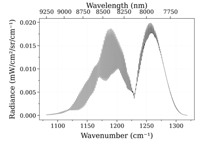
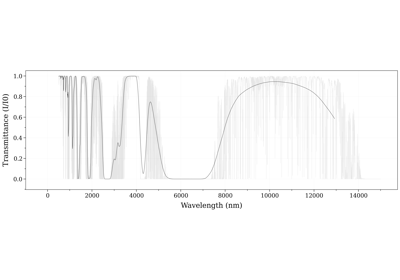
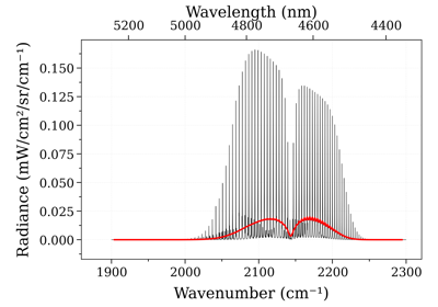
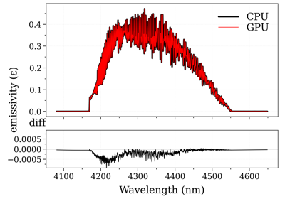
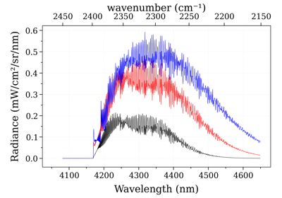

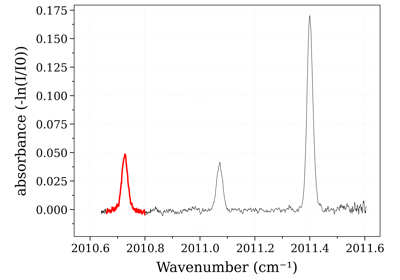

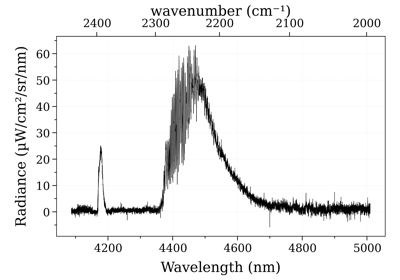
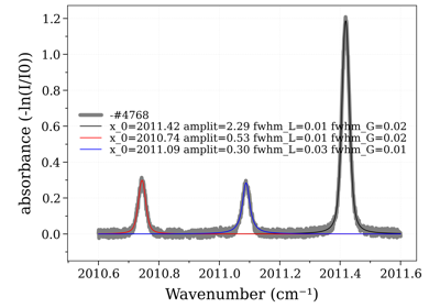

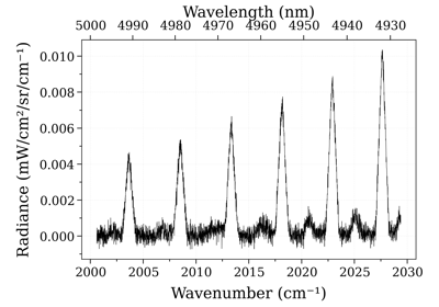
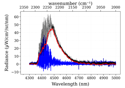
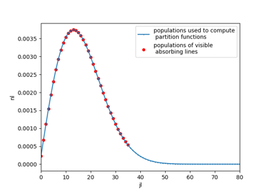


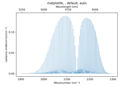
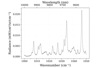
- class SpectrumFactory(wmin=None, wmax=None, wunit=cm - 1, wavenum_min=None, wavenum_max=None, wavelength_min=None, wavelength_max=None, Tref=296, pressure=1.01325, mole_fraction=1, path_length=1, wstep=0.01, isotope='all', medium='air', truncation=50, neighbour_lines=0, pseudo_continuum_threshold=0, self_absorption=True, chunksize=None, optimization='simple', folding_thresh=1e-06, zero_padding=-1, broadening_method='voigt_poly', cutoff=0, parsum_mode='full summation', verbose=True, warnings=True, species=None, save_memory=False, export_populations=None, export_lines=False, gpu_backend=None, diluent=None, lbfunc=None, potential_lowering=None, pfsource='default', **kwargs)[source]
Bases:
BandFactoryA class to put together all functions related to loading CDSD and HITRAN databases, calculating the broadenings, and summing over all the lines.
- Parameters:
wmin, wmax (
floatorQuantity) – a hybrid parameter which can stand for minimum (maximum) wavenumber or minimum (maximum) wavelength depending upon the unit accompanying it. If dimensionless,wunitis considered as the accompanying unit.wunit (
'nm','cm-1') – the unit accompanying wmin and wmax. Can only be passed with wmin and wmax. Default is"cm-1".wavenum_min, wavenum_max (
float(cm^-1)orQuantity) – minimum (maximum) wavenumber to be processed in \(cm^{-1}\). use astropy.units to specify arbitrary inverse-length units.wavelength_min, wavelength_max (
float(nm)orQuantity) – minimum (maximum) wavelength to be processed in \(nm\). This wavelength can be in'air'or'vacuum'depending on the value of the parametermedium=. use astropy.units to specify arbitrary length units.pressure (
float(bar)orQuantity) – partial pressure of gas in bar. Default1.01325(1 atm). use astropy.units to specify arbitrary pressure units. For example,1013.25 * u.mbar.mole_fraction (
float[ 0 - 1]) – species mole fraction. Default1. Note that the rest of the gas is considered to be air for collisional broadening.path_length (
float(cm)orQuantity) – path length in cm. Default1. use astropy.units to specify arbitrary length units.species (
int,str, orNone) –- For molecules:
molecule id (HITRAN format) or name. If
None, the molecule can be inferred from the database files being loaded. See the list of supported molecules inMOLECULES_LIST_EQUILIBRIUMandMOLECULES_LIST_NONEQUILIBRIUM.- For atoms:
The positive or neutral atomic species (negative ions aren’t supported). It may be given in spectroscopic notation or any form that can be converted by
to_conventional_name()
Default
None.isotope (
int,list,strof the form'1,2', or'all') – isotope idFor molecules, this is the isotopologue ID (sorted by relative density: (eg: 1: CO2-626, 2: CO2-636 for CO2) - see [HITRAN-2020] documentation for isotope list for all species.
For atoms, use the isotope number of the isotope (the total number of protons and neutrons in the nucleus) - use 0 to select rows where the isotope is unspecified, in which case the standard atomic weight from the
periodictablemodule is used when mass is required.If
'all', all isotopes in database are used (this may result in larger computation times!).Default
'all'medium (
'air','vacuum') – propagating medium when giving inputs with'wavenum_min','wavenum_max'. Does not change anything when giving inputs in wavenumber. Default'air'diluent (
strordictionary) – can be a string of a single diluent or a dictionary containing diluent name as key and its mole_fraction as value.If left unspecified, it defaults to
'air'for molecules and atomic hydrogen ‘H’ for atoms.For free electrons, use the symbol ‘e-’. Currently, only H, H2, H2, and e- are supported for atoms - any other diluents have no effect besides diluting the mole fractions of the other constituents.
- Other Parameters:
Tref (K) – Reference temperature for calculations (linestrength temperature correction). HITRAN database uses 296 Kelvin. Default 296 K
self_absorption (boolean) – Compute self absorption. If
False, spectra are optically thin. DefaultTrue.truncation (float (\(cm^{-1}\))) – Half-width over which to compute the lineshape, i.e. lines are truncated on each side after
truncation(\(cm^{-1}\)) from the line center. IfNone, use no truncation (lineshapes spread on the full spectral range). Default is50\(cm^{-1}\)Note
Large values (>
50) can induce a performance drop (computation of lineshape typically scale as \(~truncation ^2\) ). The default50was chosen to maintain a good accuracy, and still exhibit the sub-Lorentzian behavior of most lines far (few hundreds \(cm^{-1}\)) from the line center.neighbour_lines (float (\(cm^{-1}\))) – The calculated spectral range is increased (by
neighbour_linescm-1 on each side) to take into account overlaps from out-of-range lines. Default is0\(cm^{-1}\).wstep (float (cm-1) or
'auto') – Resolution of wavenumber grid. Default0.01cm-1. If'auto', it is ensured that there are slightly more points for each linewidth than the value of"GRIDPOINTS_PER_LINEWIDTH_WARN_THRESHOLD"inradis.config(~/radis.json)Note
wstep = ‘auto’ is optimized for performances while ensuring accuracy, but is still experimental in 0.9.30. Feedback welcome!
cutoff (float (~ unit of Linestrength: cm-1/(#.cm-2))) – discard linestrengths that are lower that this, to reduce calculation times.
1e-27is what is generally used to generate databases such as CDSD. If0, no cutoff. Default1e-27.parsum_mode (‘full summation’, ‘tabulation’) – how to compute partition functions, at nonequilibrium or when partition function are not already tabulated.
'full summation': sums over all (potentially millions) of rovibrational levels.'tabulation': builds an on-the-fly tabulation of rovibrational levels (500 - 4000x faster and usually accurate within 0.1%). Defaultfull summation'Note
parsum_mode= ‘tabulation’ is new in 0.9.30, and makes nonequilibrium calculations of small spectra extremely fast. Will become the default after 0.9.31.
pseudo_continuum_threshold (float) – if not
0, first calculate a rough approximation of the spectrum, then moves all lines whose linestrength intensity is less than this threshold of the maximum in a semi-continuum. Values above 0.01 can yield significant errors, mostly in highly populated areas. 80% of the lines can typically be moved in a continuum, resulting in 5 times faster spectra. If0, no semi-continuum is used. Default0.save_memory (boolean) – if
True, removes databases calculated by intermediate functions (for instance, delete the full database once the linestrength cutoff criteria was applied). This saves some memory but requires to reload the database and recalculate the linestrength for each new parameter. DefaultFalse.export_populations (
'vib','rovib',None) – if not None, store populations in Spectrum. Either store vibrational populations (‘vib’) or rovibrational populations (‘rovib’). DefaultNoneexport_lines (boolean) – if
True, saves details of all calculated lines in Spectrum. This is necessary to later useline_survey(), but can take some space. DefaultFalse.chunksize (int, or
None) – Splits the lines database in several chunks during calculation, else the multiplication of lines over all spectral range takes too much memory and slows the system down. Chunksize let you change the default chunk size. IfNone, all lines are processed directly. Usually faster but can create memory problems. DefaultNonefolding_thresh (float) – Folding is a correction procedure that is applied when the lineshape is calculated with the
fftbroadening method and the linewidth is comparable towstep, that prevents sinc(v) modulation of the lineshape. Folding continues until the lineshape intensity is belowfolding_threshold. Setting to 1 or higher effectively disables folding correction.Range: 0.0 < folding_thresh <= 1.0 Default: 1e-6
zero_padding (int) – Zero padding is used in conjunction with the
fftbroadening method to prevent circular convolution at the cost of performance. When set to -1, padding is set equal to the spectrum length, which guarantees a linear convolution.Range: 0 <= zero_padding <= len(w), or zero_padding = -1 Default: -1
broadening_method (
"voigt_poly","convolve","fft") – Available methods:"voigt_poly": polynomial approximation of a Voigt profile.This is the fastest method in most cases (default).
"convolve": independent calculation of Doppler (Gaussian) andcollisional broadening (Lorentzian), then convolution in real space. This is slower but is an exact definition of a Voigt and can be used as a reference for comparison with other methods.
"fft": fast Fourier transform convolution.Only available with
optimization="simple"oroptimization="min-RMS". Because LDM convolves all lines at once, this method is often faster than real-space convolutions on large arrays ("voigt_poly","convolve").
This SpectrumFactory parameter can be manually adjusted a posteriori with:
sf = SpectrumFactory(...)
sf.params.broadening_method = 'voigt_poly'
By default,
optimization="simple"andbroadening_method="voigt_poly".optimization (
"simple","min-RMS",None) – If either"simple"or"min-RMS"LDM optimization for lineshape calculation is used:"min-RMS": weights optimized by analytical minimization of the RMS-error (See: [Spectral-Synthesis-Algorithm])"simple": weights equal to their relative position in the grid
If
None, no lineshape interpolation is performed and the lineshape of all lines is calculated.Refer to [Spectral-Synthesis-Algorithm] for more explanation on the LDM method for lineshape interpolation.
By default,
optimization="simple"andbroadening_method="voigt_poly".warnings (bool, or one of
['warn', 'error', 'ignore'], dict) – If one of['warn', 'error', 'ignore'], set the default behaviour for all warnings. Can also be a dictionary to set specific warnings only. Example:warnings = {'MissingSelfBroadeningWarning':'ignore', 'NegativeEnergiesWarning':'ignore', 'HighTemperatureWarning':'ignore'}
See
default_warning_statusfor more information.verbose (boolean, or int) – If
False, stays quiet. IfTrue, tells what is going on. If>=2, gives more detailed messages (for instance, details of calculation times). DefaultTrue.lbfunc (callable) –
- An alternative function to be used instead of the default in calculating Lorentzian broadening, which receives the following:
df: the dataframeself.df1containing the quantities used for calculating the spectrumpressure_atm:self.pressurein units of atmospheric pressure (1.01325 bar)mole_fraction:self.input.mole_fraction, the mole fraction of the species for which the spectrum is being calculatedTgas:self.input.Tgas, gas temperature in KTref:self.input.Tref, reference temperature for calculations in Kdiluent:self._diluent, the dictionary of diluents giving the mole fraction of eachdiluent_broadening_coeff: a dictionary of the broadening coefficients for each diluentisneutral: When calculating the spectrum of an atomic species, whether or not it is neutral (alwaysNonefor molecules)
- Returns:
gamma_lb,shift- The total Lorentzian HWHM [\(cm^{-1}\)], and the shift [\(cm^{-1}\)] to be subtracted from the wavenumber array to account for lineshift. If setting the lineshift here is not desired, the 2nd return object can be anything for whichbool(shift)==FalselikeNone. gamma_lb must be array-like but can also be a vaex expression if the dataframe type is vaex.
If unspecified, the broadening is handled by default by
gamma_vald3()for atoms when using the Kurucz databank, andpressure_broadening_HWHM()for molecules.For the NIST databank, the
lbfuncparameter is compulsory as NIST doesn’t provide broadening parameters.pfsource (
string) – The source for the partition function tables for an interpolator or energy level tables for a calculator. Sources implemented so far are ‘barklem’ and ‘kurucz’ for the former, and ‘nist’ for the latter. ‘default’ is currently ‘nist’. Thepfsourcecan be changed post-initialisation using theset_atomic_partition_functions()method. See the provided example for more details.potential_lowering (float (cm-1/Zeff**2)) – The value of potential lowering, only relevant when
pfsourceis ‘kurucz’ as it depends on both temperature and potential lowering. Can be changed on the fly by settingsf.input.potential_lowering. Allowed values are typically: -500, -1000, -2000, -4000, -8000, -16000, -32000. Again, see the provided example for more details.
Examples
An example using
SpectrumFactory,load_databank(), theSpectrummethods, andunitsfrom radis import SpectrumFactory from astropy import units as u sf = SpectrumFactory(wavelength_min=4165 * u.nm, wavelength_max=4200 * u.nm, isotope='1,2', truncation=10, # cm-1 optimization=None, medium='vacuum', verbose=1, # more for more details ) sf.load_databank('HITRAN-CO2-TEST') # predefined in ~/radis.json s = sf.eq_spectrum(Tgas=300 * u.K, path_length=1 * u.cm) s.rescale_path_length(0.01) # cm s.plot('radiance_noslit', Iunit='µW/cm2/sr/nm')
Refer to the online Examples for more cases.
Examples using
radis.SpectrumFactory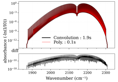
Performance increase of broadening_methods and LDM optimizations.
Performance increase of broadening_methods and LDM optimizations.
Compare OH(A-X) electronic spectra: RADIS vs Specair
Compare OH(A-X) electronic spectra: RADIS vs Specair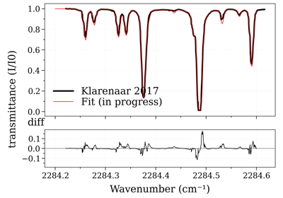
Legacy #2: non-equilibrium CO2 (Tvib_12, Tvib_3, Trot)
Legacy #2: non-equilibrium CO2 (Tvib_12, Tvib_3, Trot)
Example #7: Database fitting using SpecDatabase.fit_spectrum
Example #7: Database fitting using SpecDatabase.fit_spectrumNotes

High-level wrapper to SpectrumFactory:
Main Methods:
For advanced use:
Inputs and parameters can be accessed a posteriori with :
input: physical inputparams: computational parametersmisc: miscellaneous parameters (don’t change output)
References
See also
- df0[source]
initial line database after loading. If for any reason, you want to manipulate the line database manually (for instance, keeping only lines emitting by a particular level), you need to access the
df0attribute ofSpectrumFactory.Warning
never overwrite the
df0attribute, else some metadata may be lost in the process. Only use inplace operations. If reducing the number of lines, add a df0.reset_index()For instance:
from radis import SpectrumFactory
sf = SpectrumFactory(
    wavenum_min= 2150.4,
    wavenum_max=2151.4,
    pressure=1,
    isotope=1)
sf.load_databank('HITRAN-CO-TEST')
sf.df0.drop(sf.df0[sf.df0.vu!=1].index, inplace=True)   # keep lines emitted by v'=1 only
sf.eq_spectrum(Tgas=3000, name='vu=1').plot()
df0contains the lines as they are loaded from the database.df1is generated during the spectrum calculation, after the line database reduction steps, population calculation, and scaling of intensity and broadening parameters with the calculated conditions.See also
df1- Type:
pd.DataFrame
- df1[source]
line database, scaled with populations + linestrength cutoff Never edit manually. See all comments about
df0See also
df0- Type:
pd.DataFrame
- eq_spectrum(Tgas, mole_fraction=None, path_length=None, diluent=None, pressure=None, name=None) Spectrum[source]
Generate a spectrum at equilibrium.
- Parameters:
Tgas (float or
Quantity) – Gas temperature (K)mole_fraction (float) – database species mole fraction. If None, Factory mole fraction is used.
diluent (str or dictionary) – can be a string of a single diluent or a dictionary containing diluent name as key and its mole_fraction as value
path_length (float or
Quantity) – slab size (cm). IfNone, the default Factorypath_lengthis used.pressure (float or
Quantity) – pressure (bar). IfNone, the default Factorypressureis used.name (str) – output Spectrum name (useful in batch)
- Returns:
s –
Returns a
Spectrumobject- Return type:
Examples
- ::
from radis import SpectrumFactory sf = SpectrumFactory( wavenum_min=2900, wavenum_max=3200, molecule=”OH”, wstep=0.1, ) sf.fetch_databank(“hitemp”)
s1 = sf.eq_spectrum(Tgas=300, path_length=1, pressure=0.1) s2 = sf.eq_spectrum(Tgas=500, path_length=1, pressure=0.1)
References
See also
- eq_spectrum_gpu(Tgas, mole_fraction=None, diluent=None, path_length=None, pressure=None, name=None, backend='vulkan', device_id=0, exit_gpu=False, verbose=None) Spectrum[source]
Generate a spectrum at equilibrium with calculation of lineshapes and broadening done on the GPU.
- Parameters:
Tgas (float or
Quantity) – Gas temperature (K)mole_fraction (float) – database species mole fraction. If None, Factory mole fraction is used.
path_length (float or
Quantity) – slab size (cm). IfNone, the default Factorypath_lengthis used.pressure (float or
Quantity) – pressure (bar). IfNone, the default Factorypressureis used.name (str) – output Spectrum name (useful in batch)
- Other Parameters:
device_id (int, str) – Select the GPU device. If
int, specifies the device index, which is printed for convenience during GPU initialization with backend=’vulkan’ (default). Ifstr, return the first device that includes the specified string (case-insensitive). If not found, return the device at index 0. default = 0exit_gpu (bool) – Specifies whether the GPU app should be exited after producing the spectrum. Usually this is undesirable, because the GPU computations start to benefit after the first spectrum is produced by calling s.recalc_gpu(). See also
recalc_gpu()default = Falsebackend (str) – Since version 0.16, only
'vulkan'backend is supported. In previous versions,'gpu-cuda'and'cpu-cuda'were available to switch to a CUDA backend, but this has been deprecated in favor of the Vulkan backend... warning:: – The
backendparameter is deprecated. Only the Vulkan backend is supported.
- Returns:
s – Returns a
SpectrumobjectUse the
get()method to get something among['radiance', 'radiance_noslit', 'absorbance', etc...]Or directly the
plot()method to plot it. See [1]_ to get an overview of all Spectrum methods- Return type:
Examples
Examples using
radis.lbl.SpectrumFactory.eq_spectrum_gpu¶See also
- eq_spectrum_gpu_interactive(var='transmittance', slit_function=0.0, mpl_backend='', plotkwargs={}, *vargs, **kwargs) Spectrum[source]
- Parameters:
var (TYPE, optional) – DESCRIPTION. The default is “transmittance”.
slit_function (TYPE, optional) – DESCRIPTION. The default is 0.0.
*vargs (TYPE) – arguments forwarded to
eq_spectrum_gpu()**kwargs (dict) – arguments forwarded to
eq_spectrum_gpu()In particular, seebackend=.plotkwargs (dict) – arguments forwarded to
plot()
- Returns:
s – DESCRIPTION.
- Return type:
TYPE
Examples
from radis import SpectrumFactory
from radis.tools.plot_tools import ParamRange

sf = SpectrumFactory(2200, 2400, # cm-1
                  molecule='CO2',
                  isotope='1,2,3',
                  wstep=0.002,
                  )

sf.fetch_databank('hitemp')

s = sf.eq_spectrum_gpu_interactive(Tgas=ParamRange(300.0,2000.0,1200.0), #K
                               pressure=0.2, #bar
                               mole_fraction=0.1,
                               path_length=ParamRange(0,10,2.0), #cm
                               slit_function=ParamRange(0,1,0), #cm
                               )
- fit_legacy(s_exp, model, fit_parameters, bounds={}, plot=False, solver_options={'maxiter': 300}, **kwargs) Spectrum | OptimizeResult[source]
Fit an experimental spectrum with an arbitrary model and an arbitrary number of fit parameters. This method calls
fit_legacy()which is still functional. However, we recommend usingfit_spectrum().- Parameters:
s_exp (Spectrum) – experimental spectrum. Should have only spectral array only. Use
take(), e.g:sf.fit_legacy(s_exp.take('transmittance'))
model (func -> Spectrum) – a line-of-sight model returning a Spectrum. Example :
Tvib12Tvib3Trot_NonLTEModel()fit_parameters (dict) –
example:
{fit_parameter:initial_value}
bounds (dict, optional) –
example:
{fit_parameter:[min, max]}
fixed_parameters (dict) –
fixed parameters given to the model. Example:
fit_spectrum(fixed_parameters={"vib_distribution":"treanor"})
- Other Parameters:
plot (bool) – if
True, plot spectra as they are computed; and plot the convergence of the residual. DefaultFalsesolver_options (dict) – parameters forwarded to the solver. More info in
minimizeExample:{"maxiter": (int) max number of iteration default ``300``, }kwargs (dict) – forwarded to
fit_spectrum()
- Returns:
s_best (Spectrum) – best spectrum
res (OptimizeResults) – output of
minimize
Examples
See a one-temperature fit example and a non-LTE fit example
More advanced tools for interactive fitting of multi-dimensional, multi-slabs spectra can be found in
fitroom.See also
fit_spectrum(),Tvib12Tvib3Trot_NonLTEModel(),fitroom
- generate_perf_profile()[source]
Generate a visual/interactive performance profile diagram for the last calculated spectrum, with
tuna.Requires a
profilerkey with in Spectrum.conditions, andtunainstalled.Note
print_perf_profile()is an ascii-version which does not requiretuna.Examples
sf = SpectrumFactory(...)
sf.eq_spectrum(...)
sf.generate_perf_profile()
See typical output in https://github.com/radis/radis/pull/325
Note
You can also profile with
tunadirectly:python -m cProfile -o program.prof your_radis_script.py tuna your_radis_script.py
See also
- misc[source]
Miscellaneous parameters (
MiscParams) params that cannot change the output of calculations (ex: number of CPU, etc.)
- molparam[source]
contains information about molar mass; isotopic abundance.
See
MolParams- Type:
MolParam
- non_eq_spectrum(Tvib=None, Trot=None, Ttrans=None, Telec=None, mole_fraction=None, path_length=None, diluent=None, pressure=None, vib_distribution='boltzmann', rot_distribution='boltzmann', overpopulation=None, name=None) Spectrum[source]
Calculate emission spectrum in non-equilibrium case. Calculates absorption with broadened linestrength and emission with broadened Einstein coefficient.
- Parameters:
Tvib (float) – vibrational temperature [K] can be a tuple of float for the special case of more-than-diatomic molecules (e.g: CO2); only applicable for molecules, not atoms
Trot (float) – rotational temperature [K]; only applicable for molecules, not atoms
Ttrans (float) – translational temperature [K]. If None, translational temperature is taken as rotational temperature (valid at 1 atm for times above ~ 2ns which is the RT characteristic time)
Telec (float) – electronic temperature [K]. For molecules, see
ElectronicSpectraWarningmole_fraction (float) – database species mole fraction. If None, Factory mole fraction is used.
diluent (str or dictionary) – can be a string of a single diluent or a dictionary containing diluent name as key and its mole_fraction as value
path_length (float or
Quantity) – slab size (cm). IfNone, the default Factorypath_lengthis used.pressure (float or
Quantity) – pressure (bar). IfNone, the default Factorypressureis used.
- Other Parameters:
vib_distribution (
'boltzmann','treanor') – vibrational distributionrot_distribution (
'boltzmann') – rotational distributionoverpopulation (dict, or
None) –add overpopulation factors for given levels:
{level:overpopulation_factor}
name (str) – output Spectrum name (useful in batch)
- Returns:
s –
Returns a
Spectrumobject- Return type:
Examples
from radis import SpectrumFactory
sf = SpectrumFactory(
wavenum_min=2000,
wavenum_max=3000,
molecule="CO",
isotope="1,2,3",
wstep="auto"
)
sf.fetch_databank("hitemp", load_columns='noneq')

s1 = sf.non_eq_spectrum(Tvib=2000, Trot=600, path_length=1, pressure=0.1)
s2 = sf.non_eq_spectrum(Tvib=2000, Trot=600, path_length=1, pressure=0.1)
Multi-vibrational temperature. Below we compare non-LTE spectra of CO2 where all vibrational temperatures are equal, or where the bending and symmetric modes are in equilibrium with rotation
from radis import SpectrumFactory
sf = SpectrumFactory(
wavenum_min=2000,
wavenum_max=3000,
molecule="CO2",
isotope="1,2,3",
)
sf.fetch_databank("hitemp", load_columns='noneq')
# nonequilibrium between bending+symmetric and asymmetric modes :
s1 = sf.non_eq_spectrum(Tvib=(600, 600, 2000), Trot=600, path_length=1, pressure=1)
# all vibrational temperatures are equal :
s2 = sf.non_eq_spectrum(Tvib=(2000, 2000, 2000), Trot=600, path_length=1, pressure=1)
References
See also
- optically_thin_power(Tgas=None, Tvib=None, Trot=None, Ttrans=None, vib_distribution='boltzmann', rot_distribution='boltzmann', mole_fraction=None, path_length=None, unit='mW/cm2/sr')[source]
Calculate total power emitted in equilibrium or non-equilibrium case in the optically thin approximation: it sums all emission integral over the total spectral range.
Warning
this is a fast implementation that doesnt take into account the contribution of lines outside the given spectral range. It is valid for spectral ranges surrounded by no lines, and spectral ranges much broadened than the typical line broadening (~ 1-10 cm-1 in the infrared)
If what you’re looking for is an accurate simulation on a narrow spectral range you better calculate the spectrum (that does take all of that into account) and integrate it with
get_power()- Parameters:
Tgas (float) – equilibrium temperature [K] If doing a non equilibrium case it should be None. Use Ttrans for translational temperature
Tvib (float) – vibrational temperature [K]
Trot (float) – rotational temperature [K]
Ttrans (float) – translational temperature [K]. If None, translational temperature is taken as rotational temperature (valid at 1 atm for times above ~ 2ns which is the RT characteristic time)
mole_fraction (float) – database species mole fraction. If None, Factory mole fraction is used.
path_length (float) – slab size (cm). If None, Factory mole fraction is used.
unit (str) – output unit. Default
'mW/cm2/sr'
- Returns:
float – see
unit=.- Return type:
Returns total power density in mW/cm2/sr (unless different unit is chosen),
See also
- params[source]
Parametersthey may change the output of calculations (ex: threshold, cutoff, broadening methods, etc.)- Type:
Computational parameters
- predict_time()[source]
predict_time(self) uses the input parameters like Spectral Range, Number of lines, wstep, truncation to predict the estimated calculation time for the Spectrum broadening step(bottleneck step) for the current optimization and broadening_method. The formula for predicting time is based on benchmarks performed on various parameters for different optimization, broadening_method and deriving its time complexity.
Benchmarks: https://anandxkumar.github.io/Benchmark_Visualization_GSoC_2021/
Complexity vs Calculation Time Visualizations LBL>Voigt: LINK, DIT>Voigt: LINK, DIT>FFT: LINK
- Returns:
float
- Return type:
Predicted time in seconds.
- print_perf_profile(number_format='{:.3f}', precision=16)[source]
Prints Profiler output dictionary in a structured manner for the last calculated spectrum
Examples
sf.print_perf_profile() # output >> spectrum_calculation 0.189s ████████████████ check_line_databank 0.000s check_non_eq_param 0.042s ███ fetch_energy_5 0.015s █ calc_weight_trans 0.008s reinitialize 0.002s copy_database 0.000s memory_usage_warning 0.002s reset_population 0.000s calc_noneq_population 0.041s ███ part_function 0.035s ██ population 0.006s scaled_non_eq_linestrength 0.005s map_part_func 0.001s corrected_population_se 0.003s calc_emission_integral 0.006s applied_linestrength_cutoff 0.002s calc_lineshift 0.001s calc_hwhm 0.007s generate_wavenumber_arrays 0.001s calc_line_broadening 0.074s ██████ precompute_LDM_lineshapes 0.012s LDM_Initialized_vectors 0.000s LDM_closest_matching_line 0.001s LDM_Distribute_lines 0.001s LDM_convolve 0.060s █████ others 0.001s calc_other_spectral_quan 0.003s generate_spectrum_obj 0.000s others -0.016s- Other Parameters:
precision (int, optional) – total number of blocks. Default 16.
See also
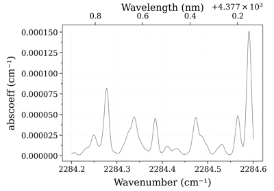


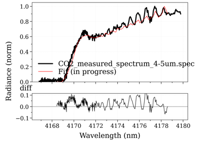
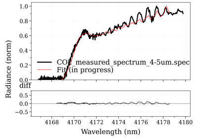
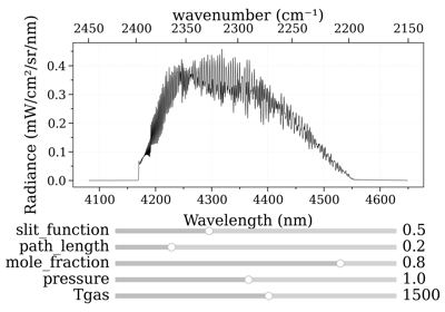
- Transmittance(s: Spectrum) Spectrum[source]
Returns a new Spectrum with only the
transmittancecomponent ofs- Parameters:
s (Spectrum) –
Spectrumobject- Returns:
s_tr –
Spectrumobject, with only thetransmittance,absorbanceand/orabscoeffpart ofs, whereradiance_noslit,emisscoeffandemissivity_noslit(if they exist) have been set to 0- Return type:
Examples
This function is useful to use Spectrum algebra operations:
s = calc_spectrum(...)   # contains emission & absorption arrays
tr = Transmittance(s)    # contains 'radiance_noslit' array only
tr -= 0.1    # arithmetic operation is applied to Transmittance only
Equivalent to:
rad = s.take('transmittance')
See also
Transmittance_noslit(),Radiance_noslit(),Radiance(),take()
- Transmittance_noslit(s: Spectrum) Spectrum[source]
Returns a new Spectrum with only the
transmittance_noslitcomponent ofs- Parameters:
s (Spectrum) –
Spectrumobject- Returns:
s_tr –
Spectrumobject, with onlytransmittance_noslitdefined- Return type:
Examples
This function is useful to use Spectrum algebra operations:
s = calc_spectrum(...)   # contains emission & absorption arrays
tr = Transmittance_noslit(s) # contains 'radiance_noslit' array only
tr -= 0.1    # arithmetic operation is applied to Transmittance_noslit only
Equivalent to:
rad = s.take('transmittance_noslit')
See also
- calc_spectrum(wmin=None, wmax=None, wunit=cm - 1, Tgas=None, Tvib=None, Trot=None, Telec=None, pressure=1.01325, species=None, isotope='all', mole_fraction=1, diluent=None, path_length=1, databank='hitran', medium='air', wstep=0.01, truncation=50, neighbour_lines=0, cutoff=1e-27, parsum_mode='full summation', optimization='simple', chunksize=None, broadening_method='voigt_poly', overpopulation=None, name=None, save_to='', use_cached=True, mode='cpu', export_lines=False, verbose=True, return_factory=False, **kwargs) Spectrum[source]
Calculate a
Spectrum.Can automatically download databases or use manually downloaded local databases, under equilibrium or non-equilibrium, with or without overpopulation, using either CPU or GPU.
It is a wrapper to
SpectrumFactoryclass. For advanced used, please refer to the aforementioned class.- Parameters:
wmin, wmax (float [\(cm^{-1}\)] or
Quantity) –wavelength/wavenumber range. If no units are given, use \(cm^{-1}\)
calc_spectrum(2000, 2300, ... )   # cm-1
calc_spectrum(4000, 4200, wunit='nm', ...)
You can use arbitrary units:
import astropy.units as u
calc_spectrum(2.5*u.um, 3.0*u.um, ...)
wunit (
'nm','cm-1','nm_air','nm_vac') – unit forwminandwmax.'nm'uses themediumparameter to determine air or vacuum conversion.'nm_air'and'nm_vac'are explicit and override themediumparameter. Default is"cm-1".Tgas (float [\(K\)]) – Gas temperature. If non equilibrium, is used for \(T_{translational}\). Default
300KTvib, Trot (float [\(K\)]) – Vibrational and rotational temperatures (for non-LTE calculations). If
None, they are at equilibrium withTgas. Only applicable for molecules, not atoms.Telec (float [\(K\)]) – Electronic temperature (for non-LTE calculations). If
None, it is at equilibrium withTgas. Only implemented for atoms, not molecules.pressure (float [\(bar\)] or
Quantity) –partial pressure of gas in bar. Default
1.01325(1 atm). Use arbitrary units:import astropy.units as u calc_spectrum(..., pressure=20*u.mbar)
species (int, str, list or
None) –- For molecules:
molecule id (HITRAN format) or name. For multiple molecules, use a list. The
'isotope','mole_fraction','databank'and'overpopulation'parameters must then be dictionaries. IfNone, the molecule can be inferred from the database files being loaded. See the list of supported molecules inMOLECULES_LIST_EQUILIBRIUMandMOLECULES_LIST_NONEQUILIBRIUM.- For atoms:
The positive or neutral atomic species. It may be given in spectroscopic notation or any form that can be converted by
to_conventional_name()
Default
None.isotope (int, list, str of the form
'1,2', or'all', or dict) – isotope idFor molecules, this is the isotopologue ID (sorted by relative density: (eg: 1: CO2-626, 2: CO2-636 for CO2) - see [HITRAN-2020] documentation for isotope list for all species.
For atoms, use the isotope number of the isotope (the total number of protons and neutrons in the nucleus) - use 0 to select rows where the isotope is unspecified, in which case the standard atomic weight from the
periodictablemodule is used when mass is required.If
'all', all isotopes in database are used (this may result in larger computation times!).Default
'all'.For multiple molecules, use a dictionary with molecule names as keys
isotope={'CO2':'1,2' , 'CO':'1,2,3' }mole_fraction (float or dict) – database species mole fraction. Default
1.For multiple molecules, use a dictionary with molecule names as keys
mole_fraction={'CO2': 0.8, 'CO':0.2}diluent (str or dictionary) – can be a string of a single diluent or a dictionary containing diluent name as key and its mole_fraction as value For single diluent
diluent = 'CO2'
For multiple diluents
diluent = { 'CO2': 0.6, 'H2O':0.2}
For free electrons, use the symbol ‘e-’. Currently, only H, H2, H2, and e- are supported for atoms - any other diluents have no effect besides diluting the mole fractions of the other constituents.
If left as
None, it defaults to'air'for molecules and atomic hydrogen ‘H’ for atoms.path_length (float [\(cm\)] or
Quantity) –slab size. Default
1cm. Use arbitrary units:import astropy.units as u calc_spectrum(..., path_length=1000*u.km)
databank (str or dict) – can be either: -
'hitran', to fetch the latest HITRAN versionthrough
fetch_hitran()(download full database with [HAPI]) orfetch_astroquery()(download only the required range). To use one mode or the other, usedatabank=('hitran', 'full') # download and cache full database, all isotopes databank=('hitran', 'range') # download and cache required range, required isotope
'hitemp', to fetch the latest HITEMP version throughfetch_hitemp(). Downloads all lines and all isotopes.'exomol', to fetch the latest ExoMol database throughfetch_exomol(). To download a specific database use (more info in fetch_exomol)databank=('exomol', 'EBJT') # 'EBJT' is a specific ExoMol database name
'geisa', to fetch the GEISA 2020 database throughfetch_geisa(). Downloads all lines and all isotopes.the name of a valid database file, in which case the format is inferred. For instance,
'.par'is recognized ashitran/hitempformat. Accepts wildcards'*'to select multiple filesdatabank='PATH/TO/co_*.par'
'kurucz'to fetch the Kurucz linelists for atoms throughfetch_kurucz(). Downloads al lines and all isotopes.'NIST'to fetch the linelists for atoms throughfetch_nist(). Downloads al lines and all isotopes.the name of a spectral database registered in your
~/radis.jsonconfiguration filedatabank='MY_SPECTRAL_DATABASE'
Default
'hitran'. SeeDatabankLoaderfor more information on line databases, andDBFORMATfor your~/radis.jsonfile format.For multiple molecules, use a dictionary with molecule names as keys:
databank='hitran'     # automatic download (or 'hitemp')
databank='PATH/TO/05_HITEMP2019.par'    # path to a file
databank='*CO2*.par' #to get all the files that have CO2 in their names (case insensitive)
databank='HITEMP-2019-CO'   # user-defined database in Configuration file
databank = {'CO2' : 'PATH/TO/05_HITEMP2019.par', 'CO' : 'hitran'}  # for multiple molecules
- Other Parameters:
medium (
'air','vacuum') – propagating medium when giving inputs with'wavenum_min','wavenum_max'. Does not change anything when giving inputs in wavenumber. Default ``’air’``wstep (float (\(cm^{-1}\)) or
'auto') – Resolution of wavenumber grid. Default0.01cm-1. If'auto', it is ensured that there are slightly more or less thanradis.config['GRIDPOINTS_PER_LINEWIDTH_WARN_THRESHOLD']points for each linewidth.Note
wstep = ‘auto’ is optimized for performances while ensuring accuracy, but is still experimental in 0.9.30. Feedback welcome!
truncation (float (\(cm^{-1}\))) – Half-width over which to compute the lineshape, i.e. lines are truncated on each side after
truncation(\(cm^{-1}\)) from the line center. IfNone, use no truncation (lineshapes spread on the full spectral range). Default is50\(cm^{-1}\)Note
Large values (>
50) can induce a performance drop (computation of lineshape typically scale as \(~truncation ^2\) ). The default50was chosen to maintain a good accuracy, and still exhibit the sub-Lorentzian behavior of most lines far (few hundreds \(cm^{-1}\)) from the line center.neighbour_lines (float (\(cm^{-1}\))) – The calculated spectral range is increased (by
neighbour_linescm-1 on each side) to take into account overlaps from out-of-range lines. Default is0\(cm^{-1}\).cutoff (float (~ unit of Linestrength: \(cm^{-1}/(molec.cm^{-2})\))) – discard linestrengths that are lower that this, to reduce calculation times.
1e-27is what is generally used to generate line databases such as CDSD. If0, no cutoff. Default1e-27.parsum_mode (‘full summation’, ‘tabulation’) – how to compute partition functions, at nonequilibrium or when partition function are not already tabulated.
'full summation': sums over all (potentially millions) of rovibrational levels.'tabulation': builds an on-the-fly tabulation of rovibrational levels (500 - 4000x faster and usually accurate within 0.1%). Default'full summation'Note
parsum_mode= ‘tabulation’ is new in 0.9.30, and makes nonequilibrium calculations of small spectra extremely fast. Will become the default after 0.9.31.
optimization (
"simple","min-RMS",None) – If either"simple"or"min-RMS"LDM optimization for lineshape calculation is used:"min-RMS": weights optimized by analytical minimization of the RMS-error (See: [Spectral-Synthesis-Algorithm])"simple": weights equal to their relative position in the grid
If using the LDM optimization, broadening method is automatically set to
'fft'. IfNone, no lineshape interpolation is performed and the lineshape of all lines is calculated. Refer to [Spectral-Synthesis-Algorithm] for more explanation on the LDM method for lineshape interpolation. Default"simple".overpopulation (dict) – dictionary of overpopulation compared to the given vibrational temperature. Default
None. Example:overpopulation = {'CO2' : {'(00`0`0)->(00`0`1)': 2.5, '(00`0`1)->(00`0`2)': 1, '(01`1`0)->(01`1`1)': 1, '(01`1`1)->(01`1`2)': 1 } }export_lines (boolean) – if
True, saves details of all calculated lines in Spectrum. This is necessary to later useline_survey(), but can take some space. DefaultFalse.name (str) – name of the output Spectrum. If
None, a unique ID is generated.save_to (str) – save to a
specfile which contains absorption & emission features, all calculation parameters, and can be opened withload_spec(). File can be reloaded and exported to text formats afterwards, seesavetxt(). If file already exists, replace.use_cached (boolean) – use cached files for line database and energy database. Default
True.verbose (boolean, or int) – If
False, stays quiet. IfTrue, tells what is going on. If>=2, gives more detailed messages (for instance, details of calculation times). DefaultTrue.mode (
'cpu','gpu') – if set to'cpu', computes the spectra purely on the CPU. if set to'gpu', offloads the calculations of lineshape and broadening steps to the GPU making use of parallel computations to speed up the process. GPU computations initiated in this way will use the Vulkan backend; useSpectrumFactoryfor more flexibility. GPU spectra will be returned with exit_gpu=False, so the user should call Spectrum.gpu_exit() when they’re done with GPU computations. Only'cpu'is available for atoms. Default'cpu'.return_factory (bool) – if
True, return theSpectrumFactorythat computes the spectrum. Useful to access computational parameters, the line database, or to start batch-computations from a first spectrum calculation. Ex:s, sf = calc_spectrum(..., return_factory=True, save_memory=False) sf.df1 # see the lines calculated sf.eq_spectrum(...) # new calculation without reloading the database
**kwargs (other inputs forwarded to SpectrumFactory) – For instance:
warnings. SeeSpectrumFactorydocumentation for more details on input.
- Returns:
Spectrum– Output spectrum:SpectrumFactory– if usingreturn_factory=True, the Factory that generated the spectrum is returned. if calculating multiple molecules, a dictionary of factories is returned
References
.. [2] RADIS GPU support: GPU Calculations on RADIS
Examples
Calculate a CO spectrum from the HITRAN database:
from radis import calc_spectrum
s = calc_spectrum(1900, 2300,         # cm-1
                  molecule='CO',
                  isotope='1,2,3',
                  pressure=1.01325,   # bar
                  Tgas=1000,
                  mole_fraction=0.1,
                  databank='hitran',  # or 'hitemp'
                  diluent = "air"     # or {'CO2': 0.1, 'air':0.8}
                  )
s.apply_slit(0.5, 'nm')
s.plot('radiance')
This example uses the
apply_slit()andplot()methods. See alsoline_survey():s.line_survey(overlay='radiance')
Calculate a CO2 spectrum from the CDSD-4000 database:
T_list = [1000.0, 1500.0, 2000.0]
s = calc_spectrum(2200, 2400,   # cm-1
                  molecule='CO2',
                  isotope='1',
                  databank='/path/to/cdsd/databank/in/npy/format/',
                  pressure=0.1,  # bar
                  Tgas=T_list[0],
                  mole_fraction=0.1,
                  mode='gpu',
                  )
s.plot('absorbance', show=False)

for T in T_list[1:]:
    s.recalc_gpu(Tgas=T)
    show = (True if T == T_list[-1] else False)
    s.plot("absorbance", show=show, nfig="same")

s.exit_gpu()
This example uses the
eq_spectrum_gpu()method to calculate the spectrum on the GPU. The databank points to the CDSD-4000 databank that has been pre-processed and stored innumpy.npyformat. Consecutive spectra are calulated using the s.recalc_gpu() method, which uses the GPU to rapidly speed up calculations. Without using consecutive s.recalc_gpu() calls, GPU computations do not provide significant advantage to CPU mode. Refer to the online Examples for more cases, and to the Spectrum page for details on post-processing methods.For more details on how to use the GPU method and process the database, refer to the examples linked above and the documentation on GPU support for RADIS. Other Examples ————–
Calculate and Compare Spectra for Multiple Molecules
Calculate and Compare Spectra for Multiple MoleculesReferences
cite: RADIS is built on the shoulders of many state-of-the-art packages and databases. If using RADIS to compute spectra, make sure you cite all of them, for proper reproducibility and acknowledgement of the work ! See How to cite? and the
cite()method.See also

- calculated_spectrum(w, I, wunit='nm', Iunit='mW/cm2/sr/nm', conditions=None, cond_units=None, populations=None, name=None) Spectrum[source]
Convert
(w, I)into aSpectrumobject that has unit conversion, plotting and slit convolution capabilities.- Parameters:
w (np.array) – wavelength, or wavenumber
I (np.array) – intensity (no slit)
wunit (
'nm','cm-1','nm_vac') – wavespace unit: wavelength in air ('nm'), wavenumber ('cm-1'), or wavelength in vacuum ('nm_vac'). Default'nm'.Iunit (str) – intensity unit (can be ‘counts’, ‘mW/cm2/sr/nm’, etc…). Default ‘mW/cm2/sr/nm’ (note that non-convoluted Specair spectra are in ‘mW/cm2/sr/µm’)
- Other Parameters:
conditions (dict) – (optional) calculation conditions to be stored with Spectrum. Default
Nonecond_units (dict) – (optional) calculation conditions units. Default
Nonepopulations (dict) – populations to be stored in Spectrum. Default
Nonename (str) – (optional) give a name
Examples
# w, I are numpy arrays for wavelength and radiance
from radis import calculated_spectrum
s = calculated_spectrum(w, I, wunit='nm', Iunit='W/cm2/sr/nm')     # creates 'radiance_noslit'
- cdsd2df(fname, version='hitemp', cache=True, load_columns=None, verbose=True, drop_non_numeric=True, load_wavenum_min=None, load_wavenum_max=None, engine='pytables', output='pandas')[source]
Convert a CDSD-HITEMP [1]_ or CDSD-4000 [2]_ file to a Pandas dataframe.
- Parameters:
fname (str) – CDSD file name
version (str (‘4000’, ‘hitemp’)) – CDSD version
cache (boolean, or ‘regen’) – if
True, a pandas-readable HDF5 file is generated on first access, and later used. This saves on the datatype cast and conversion and improves performances a lot (but changes in the database are not taken into account). IfFalse, no database is used. If ‘regen’, temp file are reconstructed. DefaultTrue.load_columns (list) – columns to load. If
None, loads everythingNote
this is only relevant if loading from a cache file. To generate the cache file, all columns are loaded anyway.
- Other Parameters:
drop_non_numeric (boolean) – if
True, non numeric columns are dropped. This improves performances, but make sure all the columns you need are converted to numeric formats before hand. DefaultTrue. Note that if a cache file is loaded it will be left untouched.load_wavenum_min, load_wavenum_max (float) – if not
'None', only load the cached file if it contains data for wavenumbers above/below the specified value. See :py:func`~radis.api.cache_files.load_h5_cache_file`. Default'None'.engine (‘pytables’, ‘vaex’) – format for Hdf5 cache file. Default
pytables
- Returns:
df – dataframe containing all lines and parameters
- Return type:
pandas Dataframe or Vaex Dataframe
Notes
CDSD-4000 Database can be downloaded from [3]
Performances: I had huge performance trouble with this function, because the files are huge (500k lines) and the format is to special (no space between numbers…) to apply optimized methods such as pandas’s. A line by line reading isn’t so bad, using struct to parse each line. However, we waste typing determining what every line is. I ended up using the fromfiles functions from numpy, not considering n (line return) as a special character anymore, and a second call to numpy to cast the correct format. That ended up being twice as fast.
initial: 20s / loop
with mmap: worse
w/o readline().rstrip(’n’): still 20s
numpy fromfiles: 17s
no more readline, 2x fromfile 9s
Think about using cache mode too:
no cache mode 9s
cache mode, first time 22s
cache mode, then 2s
Moving to HDF5:
On cdsd_02069_02070 (56 Mb)
Reading:
cdsd2df(): 9.29 s
cdsd2df(cache=True [old .txt version]): 2.3s
cdsd2df(cache=True [new h5 version, table]): 910ms
cdsd2df(cache=True [new h5 version, fixed]): 125ms
Storage:
%timeit df.to_hdf("cdsd_02069_02070.h5", "df", format="fixed")  337ms
%timeit df.to_hdf("cdsd_02069_02070.h5", "df", format="table")  1.03s
References
Note that CDSD-HITEMP is used as the line database for CO2 in HITEMP 2010
See also
hit2df()
- config = {'ALLOW_OVERWRITE': True, 'AUTO_UPDATE_DATABASE': False, 'AUTO_UPDATE_SPEC': False, 'DATAFRAME_ENGINE': 'pandas', 'DEBUG_MODE': False, 'DEFAULT_DOWNLOAD_PATH': '~/.radisdb', 'GRIDPOINTS_PER_LINEWIDTH_ERROR_THRESHOLD': 1, 'GRIDPOINTS_PER_LINEWIDTH_WARN_THRESHOLD': 3, 'MEMORY_MAPPING_ENGINE': 'auto', 'MISSING_BROAD_COEF': 'air', 'OLDEST_COMPATIBLE_VERSION': '0.9.1', 'RESAMPLING_TOLERANCE_THRESHOLD': 0.005, 'SPARSE_WAVERANGE': 'auto', 'WARN_LARGE_DOWNLOAD_ABOVE_X_GB': 1, '_HELLO!': 'This is your RADIS configuration file. Any key here will overwrite the values of the radis/default_radis.json file on your local computer (see online version of the latest release: https://github.com/radis/radis/blob/master/radis/default_radis.json). More information on the online docs : https://radis.readthedocs.io/en/latest/lbl/lbl.html#label-lbl-config-file', 'database': {}, 'plot': {'context': 'poster', 'plotlib': 'publib', 'plotting_library': 'auto', 'style': 'origin'}, 'plotting_library': 'auto', 'spectroscopic_constants': {'CO': 'molecules_data.json', 'CO2': 'molecules_data.json'}}[source]
RADIS configuration parameters
- Parameters:
“DEBUG_MODE” (False) –
bool: change this at runtime with:
import radis
radis.config["DEBUG_MODE"] = True
Use the
printdbg()function inradis.misc, typically with:if __debug__: printdbg(...)
so that printdbg are removed by the Python preprocessor when running in optimize mode:
python -O *.py
“ALLOW_OVERWRITE” (False) – bool: Whether to allow RADIS to overwrite values of a databank entry that is already registered. If True, allow RADIS to download files and make changes to the local database folder even when the databank is already registered, and then re-register it with the values for the new files, overwriting the previously registered values. This could occur when e.g. running
fetch_databankwith thecacheargument set to “regen” or the registered “paths” not including the path to the databank itself or some of the registered files missing from the disk, resulting in files being re-downloaded and the “download_date” (and possibly “paths”) value being updated. If False, no changes are made to the local database folder when a databank is already registered, and an exception is raised in cases where re-registering would have been required, so e.g. in the example above, this setting would prevent the “download_date” from being updated and hence an exception would be raised instead. False by default, so RADIS only ever inserts new databank entries and doesn’t modify existing ones, hence a databank entry is only ever modified by the user and responsibility is on them to ensure it is adequate for the code to run as RADIS wouldn’t automatically take steps to rectify inadequate entries.“AUTO_UPDATE_SPEC” (False) – bool: experimental feature used to autoupdate .spec files to the latest format, by simply saving them again once they’re loaded and fixed. Warning! Better have a copy of your files before that, or a way to regenerate them.
Example : Add to the top of your script (once is enough!):
import radis
radis.config["AUTO_UPDATE_SPEC"] = True
You can also see:
_update_to_latest_format()
- “AUTO_UPDATE_DATABASE”: False
bool: experimental feature used to autoupdate .h5 files to the latest format, by simply saving them again once they’re loaded and fixed. Warning! Better have a copy of your files before that, or a way to regenerate them.
Example. Add to the top of your script (once is enough!):
import radis
radis.AUTO_UPDATE_DATABASE = True
“MISSING_BROAD_COEF” : False
str: Accepted values: False (default) and “air”. If “air”, missing boradening coefficients are replaced by those of air.
_calc_broadening_HWHM()- “OLDEST_COMPATIBLE_VERSION”: “0.9.1”
str: forces to regenerate cache files that were created in a previous version
- “GRIDPOINTS_PER_LINEWIDTH_WARN_THRESHOLD”: 3
float: to determine the optimal value of wstep using minimum FWHM value of spectrum. Makes sure there are enough gridpoints per line.
See more in :
radis.lbl.broadening.BroadenFactory._check_accuracy()- “GRIDPOINTS_PER_LINEWIDTH_ERROR_THRESHOLD”: 1
float: to determine the minimum feasible value of wstep using minimum FWHM value of spectrum. Makes sure there are enough gridpoints per line.
See more in :
radis.lbl.broadening.BroadenFactory._check_accuracy()- “SPARSE_WAVERANGE”: True
bool: if True, allow special optimizations to improve performances for large spectra that are sparse, i.e there are no lines within
truncationdistance. In that case, spectral calculations can be an order of magnitude faster, and result in less memory use. This optimization may result in a small but unnecessary overhead when there are lines everywhere in the spectral range considered. In such cases, you may deactivate it by settingradis.config['SPARSE_WAVERANGE'] = FalseDefaultTrueSee more in
radis.lbl.broadening.BroadenFactory._apply_lineshape_LDM()- “RESAMPLING_TOLERANCE_THRESHOLD” 5e-3
an error if raises if areas do not match by a value above this threshold, during resampling. See
resample()Default
5e-3
Notes
Default values are read from the radis/default_radis.json file.
All values are overridden at runtime by the keys in the user JSON file
~/radis.json (json)(in particular, the list of databases)See more in the Configuration file documentation.
- Type:
dict
- experimental_spectrum(w, I, wunit='nm', Iunit='count', conditions={}, cond_units=None, name=None) Spectrum[source]
Convert
(w, I)into aSpectrumobject that has unit conversion and plotting capabilities. Convolution is not available as the spectrum is assumed to have be measured experimentally (hence it is already convolved with the slit function)- Parameters:
w (np.array) – wavelength, or wavenumber
I (np.array) – intensity
wunit (
'nm','cm-1','nm_vac') – wavespace unit: wavelength in air ('nm'), wavenumber ('cm-1'), or wavelength in vacuum ('nm_vac'). Default'nm'.Iunit (str) – intensity unit (can be
'count', ‘mW/cm2/sr/nm’, etc…). Default'count'(i.e., non calibrated output)
- Other Parameters:
conditions (dict) – (optional) calculation conditions to be stored with Spectrum
cond_units (dict) – (optional) calculation conditions units
name (str) – (optional) give a name
Examples
Load and plot an experimental spectrum:
from numpy import loadtxt
from radis import experimental_spectrum
w, I = loadtxt('my_file.txt').T    # transpose is often useful, depending on your data.
s = experimental_spectrum(w, I, Iunit='mW/cm2/sr/nm')             # creates 'radiance'
s.plot()
- fetch_astroquery(molecule, isotope, wmin, wmax, verbose=True, cache=True, expected_metadata={}, engine='pytables-fixed', output='pandas')[source]
Download a HITRAN line database to a Pandas DataFrame.
Wrapper to the fetch function of Astroquery [1]_ (itself based on [HAPI])
Note
if using, cite [HAPI] and [HITRAN-2020]
- Parameters:
molecule (str, or int) – molecule name or identifier
isotope (int) – isotope number
wmin, wmax (float (cm-1)) – wavenumber min and max
- Other Parameters:
verbose (boolean) – Default
Truecache (boolean or
'regen') – ifTrue, tries to find a.h5cache file in the Astroquerycache_location, that would match the requirements. If not found, downloads it and saves the line dataframe as a.h5file in the Astroquery. If'regen', delete existing cache file to regenerate it.expected_metadata (dict) – if
cache=True, check that the metadata in the cache file correspond to these attributes. Argumentsmolecule,isotope,wmin,wmaxare already added by default.output (str) – specifies the type of returned data
References
See also
astroquery.hitran.core.Hitran.query_lines_async(),astroquery.query.BaseQuery.cache_location
- fetch_exomol(molecule, database=None, local_databases=None, databank_name='EXOMOL-{molecule}', isotope='1', load_wavenum_min=None, load_wavenum_max=None, columns=None, cache=True, verbose=True, clean_cache_files=True, return_local_path=False, return_partition_function=False, engine='default', output='pandas', skip_optional_data=True, parallel=True, **kwargs)[source]
Stream ExoMol file from EXOMOL website. Unzip and build a HDF5 file directly.
Returns a Pandas DataFrame containing all lines.
- Parameters:
molecule (
str) – ExoMol moleculedatabase (
str) – database name. Ex:POKAZATELorBT2forH2O. SeeKNOWN_EXOMOL_DATABASE_NAMES. IfNoneand there is only one database available, use it. If multiple databases are available but none is recommended by ExoMol (e.g., for13C-16O), aKeyErroris raised and you must explicitly choose one.local_databases (
str) – where to create the RADIS HDF5 files. Default"~/.radisdb/exomol". Can be changed inradis.config["DEFAULT_DOWNLOAD_PATH"]or in ~/radis.json config filedatabank_name (
str) – name of the databank in RADIS Configuration file Default"EXOMOL-{molecule}"isotope (
strorint) – load only certain isotopes, sorted by terrestrial abundances :'1','2', etc. Default1.Note
In RADIS, isotope abundance is included in the line intensity calculation. However, the terrestrial abundances used may not be relevant to non-terrestrial applications. By default, the abundance is given reading HITRAN data. If the molecule does not exist in the HITRAN database, the abundance is read from the
radis/radis_default.jsonconfiguration file, which can be modified by editingradis.configafter import or directly by editing the user~/radis.jsonuser configuration file (overwritesradis_default.json). In theradis/radis_default.jsonfile, values were calculated with a simple model based on the terrestrial isotopic abundance of each element.load_wavenum_min, load_wavenum_max (float (cm-1)) – load only specific wavenumbers.
columns (list of str) – list of columns to load. If
None, returns all columns in the file.
- Other Parameters:
parallel (bool) – if True, downloads files concurrently using a thread pool, significantly speeding up the fetching process especially for databases with many transition files. Default is True.
cache (bool, or
'regen'or'force') – ifTrue, use existing HDF5 file. IfFalseor'regen', rebuild it. If'force', crash if not cache file found. DefaultTrue.verbose (bool)
clean_cache_files (bool) – if
Trueclean downloaded cache files after HDF5 are created.return_local_path (bool) – if
True, also returns the path of the local database file.return_partition_function (bool) – if
True, also returns aPartFuncExoMolobject.engine (‘vaex’, ‘feather’) – which memory-mapping library to use. If ‘default’ use the value from ~/radis.json
output (‘pandas’, ‘vaex’, ‘jax’) – format of the output DataFrame. If
'jax', returns a dictionary of jax arrays. If'vaex', output is avaex.dataframe.DataFrameLocalNote
Vaex DataFrames are memory-mapped. They do not take any space in RAM and are extremely useful to deal with the largest databases.
skip_optional_data (bool) – If False, fetch all fields which are marked as available in the ExoMol definition file. If True, load only the first 4 columns of the states file (“i”, “E”, “g”, “J”). The structure of the columns above 5 depend on the the definitions file (
*.def) and the Exomol version. Ifskip_optional_data=False, two errors may occur:a field is marked as present/absent in the
*.deffield but is absent/present in the*.statesfile (ie both files are inconsistent).in the updated version of Exomol, new fields have been added in the states file of some species. But it has not been done for all species, so both structures exist. For instance, the states file of https://exomol.com/data/molecules/HCl/1H-35Cl/HITRAN-HCl/ follows the structure described in [1]_, unlike the states file of https://exomol.com/data/molecules/NO/14N-16O/XABC/ which follows the structure described in [2]_.
- Returns:
df (pd.DataFrame or vaex.dataframe.DataFrameLocal) – Line list A HDF5 file is also created in
local_databasesand referenced in the RADIS config file with namedatabank_namelocal_path (str) – path of local database file if
return_local_path
Examples
Notes
if using
load_only_wavenum_above/beloworisotope, the whole database is anyway downloaded and uncompressed tolocal_databasesfast access .HDF5 files (which will take a long time on first call). Only the expected wavenumber range & isotopes are returned. The .HFD5 parsing useshdf2df()References
See also
- fetch_geisa(molecule, local_databases=None, databank_name='GEISA-{molecule}', isotope=None, load_wavenum_min=None, load_wavenum_max=None, columns=None, cache=True, verbose=True, chunksize=100000, clean_cache_files=True, return_local_path=False, engine='default', output='pandas', parallel=True)[source]
Stream GEISA file from GEISA website. Unzip and build a HDF5 file directly.
Returns a Pandas DataFrame containing all lines.
- Parameters:
molecule (all 58 GEISA 2020 molecules. See here https://geisa.aeris-data.fr/interactive-access/?db=2020&info=ftp)
local_databases (str) – where to create the RADIS HDF5 files. Default
"~/.radisdb/geisa". Can be changed inradis.config["DEFAULT_DOWNLOAD_PATH"]or in ~/radis.json config filedatabank_name (str) – name of the databank in RADIS Configuration file Default
"GEISA-{molecule}"isotope (str, int or None) – load only certain isotopes :
'2','1,2', etc. IfNone, loads everything. DefaultNone.load_wavenum_min, load_wavenum_max (float (cm-1)) – load only specific wavenumbers.
columns (list of str) – list of columns to load. If
None, returns all columns in the file.
- Other Parameters:
cache (
True,False,'regen'or'force') – ifTrue, use existing HDF5 file. IfFalseor'regen', rebuild it. If'force', raise an error if cache file cannot be used (useful for debugging). DefaultTrue.verbose (bool)
chunksize (int) – number of lines to process at a same time. Higher is usually faster but can create Memory problems and keep the user uninformed of the progress.
clean_cache_files (bool) – if
Trueclean downloaded cache files after HDF5 are created.return_local_path (bool) – if
True, also returns the path of the local database file.engine (‘pytables’, ‘vaex’, ‘default’) – which HDF5 library to use to parse local files. If ‘default’ use the value from ~/radis.json
output (‘pandas’, ‘vaex’, ‘jax’) – format of the output DataFrame. If
'jax', returns a dictionary of jax arrays.parallel (bool) – if
True, uses joblib.parallel to load database with multiple processes
- Returns:
df (pd.DataFrame or vaex.dataframe.DataFrameLocal) – Line list A HDF5 file is also created in
local_databasesand referenced in the RADIS config file with namedatabank_namelocal_path (str) – path of local database file if
return_local_path
Examples
from radis import fetch_geisa
df = fetch_geisa("CO")
print(df.columns)
>>> Index(['wav', 'int', 'airbrd', 'El', 'globu', 'globl', 'locu', 'locl',
    'Tdpgair', 'isoG', 'mol', 'idG', 'id', 'iso', 'A', 'selbrd', 'Pshft',
    'Tdpair', 'ierrA', 'ierrB', 'ierrC', 'ierrF', 'ierrO', 'ierrR', 'ierrN',
    'Tdpgself', 'ierrS', 'Pshfts', 'ierrT', 'Tdppself', 'ierrU'],
    dtype='object')
Notes
if using
load_only_wavenum_above/beloworisotope, the whole database is anyway downloaded and uncompressed tolocal_databasesfast access .HDF5 files (which will take a long time on first call). Only the expected wavenumber range & isotopes are returned. The .HFD5 parsing useshdf2df()if a registered entry already exists and
radis.config["ALLOW_OVERWRITE"]isTrue: - if any situation arises where the databank needs to be re-downloaded, the possible urls are attempted in their usual order of preference, as if the databank hadn’t been registered, rather than directly re-downloading from the same url that was previously registered, in case e.g. a new linelist has been uploaded since the databank was previously registered - If no partition function file is registered, e.g because one wasn’t available server-side when the databank was last registered, an attempt is still made again to download it, to account for e.g. the case where one has since been uploaded
- fetch_hitemp(molecule, local_databases=None, databank_name='HITEMP-{molecule}', isotope=None, load_wavenum_min=None, load_wavenum_max=None, columns=None, cache=True, verbose=True, chunksize=100000, clean_cache_files=True, return_local_path=False, engine='default', output='pandas', parallel=True, database='most_recent')[source]
Stream HITEMP file from HITRAN website. Unzip and build a HDF5 file directly.
Returns a Pandas DataFrame containing all lines.
- Parameters:
molecule (
"H2O", "CO2", "N2O", "CO", "CH4", "NO", "NO2", "OH") – HITEMP molecule. See https://hitran.org/hitemp/local_databases (str) – where to create the RADIS HDF5 files. Default
"~/.radisdb/hitemp". Can be changed inradis.config["DEFAULT_DOWNLOAD_PATH"]or in ~/radis.json config filedatabank_name (str) – name of the databank in RADIS Configuration file Default
"HITEMP-{molecule}"isotope (str, int or None) – load only certain isotopes :
'2','1,2', etc. IfNone, loads everything. DefaultNone.load_wavenum_min, load_wavenum_max (float (cm-1)) – load only specific wavenumbers.
columns (list of str) – list of columns to load. If
None, returns all columns in the file.
- Other Parameters:
cache (
True,False,'regen'or'force') – ifTrue, use existing HDF5 file. IfFalseor'regen', rebuild it. If'force', raise an error if cache file cannot be used (useful for debugging). DefaultTrue.verbose (bool)
chunksize (int) – number of lines to process at a same time. Higher is usually faster but can create Memory problems and keep the user uninformed of the progress.
clean_cache_files (bool) – if
Trueclean downloaded cache files after HDF5 are created.return_local_path (bool) – if
True, also returns the path of the local database file.engine (‘pytables’, ‘vaex’, ‘default’) – which HDF5 library to use to parse local files. If ‘default’ use the value from ~/radis.json
output (‘pandas’, ‘vaex’, ‘jax’) – format of the output DataFrame. If
'jax', returns a dictionary of jax arrays. If'vaex', output is avaex.dataframe.DataFrameLocalNote
Vaex DataFrames are memory-mapped. They do not take any space in RAM and are extremely useful to deal with the largest databases.
parallel (bool) – if
True, uses joblib.parallel to load database with multiple processesdatabase (
str) – The database version to retrieve. Options include: -"most_recent": Fetches the latest available database version. - A four-digit year (e.g.,"2010"): Selects a specific version, such as the 2010 or 2019 database for CO.If not provided, the default is
"most_recent".
- Returns:
df (pd.DataFrame) – Line list A HDF5 file is also created in
local_databasesand referenced in the RADIS config file with namedatabank_namelocal_path (str) – path of local database file if
return_local_path
Examples
from radis import fetch_hitemp
df = fetch_hitemp("CO")
print(df.columns)
>>> Index(['id', 'iso', 'wav', 'int', 'A', 'airbrd', 'selbrd', 'El', 'Tdpair',
    'Pshft', 'ierr', 'iref', 'lmix', 'gp', 'gpp', 'Fu', 'branch', 'jl',
    'syml', 'Fl', 'vu', 'vl'],
    dtype='object')
Notes
if using
load_only_wavenum_above/beloworisotope, the whole database is anyway downloaded and uncompressed tolocal_databasesfast access .HDF5 files (which will take a long time on first call). Only the expected wavenumber range & isotopes are returned. The .HFD5 parsing useshdf2df()if a registered entry already exists and
radis.config["ALLOW_OVERWRITE"]isTrue: - if any situation arises where the databank needs to be re-downloaded, the possible urls are attempted in their usual order of preference, as if the databank hadn’t been registered, rather than directly re-downloading from the same url that was previously registered, in case e.g. a new linelist has been uploaded since the databank was previously registered - If no partition function file is registered, e.g because one wasn’t available server-side when the databank was last registered, an attempt is still made again to download it, to account for e.g. the case where one has since been uploadedSee also
fetch_hitran(),fetch_exomol(),fetch_geisa(),fetch_kurucz(),hdf2df(),fetch_databank()
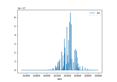
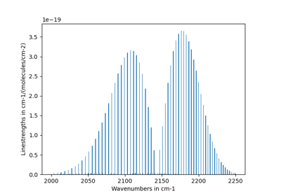
- fetch_hitran(molecule, extra_params=None, local_databases=None, databank_name='HITRAN-{molecule}', isotope=None, load_wavenum_min=None, load_wavenum_max=None, columns=None, cache=True, verbose=True, clean_cache_files=True, return_local_path=False, engine='default', output='pandas', parallel=True, parse_quanta=True)[source]
Download all HITRAN lines from HITRAN website. Unzip and build a HDF5 file directly.
Returns a Pandas DataFrame containing all lines.
- Parameters:
molecule (str) – one specific molecule name, listed in HITRAN molecule metadata. See https://hitran.org/docs/molec-meta/ Example: “H2O”, “CO2”, etc.
local_databases (str) – where to create the RADIS HDF5 files. Default
"~/.radisdb/hitran". Can be changed inradis.config["DEFAULT_DOWNLOAD_PATH"]or in ~/radis.json config filedatabank_name (str) – name of the databank in RADIS Configuration file Default
"HITRAN-{molecule}"isotope (str) – load only certain isotopes :
'2','1,2', etc. IfNone, loads everything. DefaultNone.load_wavenum_min, load_wavenum_max (float (cm-1)) – load only specific wavenumbers.
columns (list of str) – list of columns to load. If
None, returns all columns in the file.extra_params (‘all’ or None) – Downloads all additional columns available in the HAPI database for the molecule including parameters like
gamma_co2,n_co2that are required to calculate spectrum in co2 diluent. For eg:from radis.io.hitran import fetch_hitran df = fetch_hitran('CO', extra_params='all', cache='regen') # cache='regen' to regenerate new database with additional columns
- Other Parameters:
cache (
True,False,'regen'or'force') – ifTrue, use existing HDF5 file. IfFalseor'regen', rebuild it. If'force', raise an error if cache file cannot be used (useful for debugging). DefaultTrue.verbose (bool)
clean_cache_files (bool) – if
Trueclean downloaded cache files after HDF5 are created.return_local_path (bool) – if
True, also returns the path of the local database file.engine (‘pytables’, ‘vaex’, ‘default’) – which HDF5 library to use. If ‘default’ use the value from ~/radis.json
output (‘pandas’, ‘vaex’, ‘jax’) – format of the output DataFrame. If
'jax', returns a dictionary of jax arrays. If'vaex', output is avaex.dataframe.DataFrameLocalNote
Vaex DataFrames are memory-mapped. They do not take any space in RAM and are extremely useful to deal with the largest databases.
parallel (bool) – if
True, uses joblib.parallel to load database with multiple processesparse_quanta (bool) – if
True, parse local & global quanta (required to identify lines for non-LTE calculations ; but sometimes lines are not labelled.)
- Returns:
df (pd.DataFrame or vaex.dataframe.DataFrameLocal) – Line list A HDF5 file is also created in
local_databasesand referenced in the RADIS config file with namedatabank_namelocal_path (str) – path of local database file if
return_local_path
Examples
from radis.io.hitran import fetch_hitran
df = fetch_hitran("CO")
print(df.columns)
>>> Index(['id', 'iso', 'wav', 'int', 'A', 'airbrd', 'selbrd', 'El', 'Tdpair',
    'Pshft', 'gp', 'gpp', 'branch', 'jl', 'vu', 'vl'],
    dtype='object')
Notes
if using
load_only_wavenum_above/beloworisotope, the whole database is anyway downloaded and uncompressed tolocal_databasesfast access .HDF5 files (which will take a long time on first call). Only the expected wavenumber range & isotopes are returned. The .HFD5 parsing useshdf2df()if a registered entry already exists and
radis.config["ALLOW_OVERWRITE"]isTrue: - if any situation arises where the databank needs to be re-downloaded, the possible urls are attempted in their usual order of preference, as if the databank hadn’t been registered, rather than directly re-downloading from the same url that was previously registered, in case e.g. a new linelist has been uploaded since the databank was previously registered - If no partition function file is registered, e.g because one wasn’t available server-side when the databank was last registered, an attempt is still made again to download it, to account for e.g. the case where one has since been uploaded
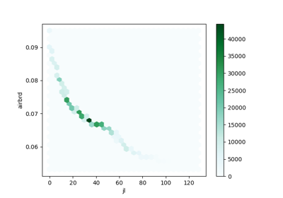
- getMolecule(molecule, isotope=None, electronic_state=None, verbose=True) ElectronicState[source]
Get an
ElectronicStateobject in the RADISMoleculeslist, which use the defaults spectroscopic constants.- Parameters:
molecule (str) – molecule name
isotope (int, or
None) – isotope number. if None, only one isotope must exist in database. Else, an error is raisedelectronic_state (str) – if None, only one electronic state must exist in database. Else, an error is raised
verbose (boolean) – if
True, print which electronic state we got
- Returns:
ElectronicState
- Return type:
an
ElectronicStateobject.
Examples
Get rovibrational energies using the default spectroscopic constants:
from radis import getMolecule

# Here we get the energy of the v=6, J=3 level of the 2nd isotope of CO:

CO = getMolecule("CO", 2, "X")
print(CO.Erovib(6, 3))
See also

- get_FWHM(w, I, return_index=False)[source]
Calculate full width half maximum (FWHM) by comparing amplitudes
- Parameters:
w, I (arrays)
return_index (boolean) – if True, returns indexes for half width boundaries. Default
False
- Returns:
FWHM (float) – full width at half maximum
[xmin, xmax] (int)
- get_diff(s1: Spectrum, s2: Spectrum, var, wunit='default', Iunit='default', resample=True, diff_window=0)[source]
Get the difference between 2 spectra.
Basically returns w1, I1 - I2 where (w1, I1) and (w2, I2) are the values of s1 and s2 for variable var. (w2, I2) is linearly interpolated if needed.
\[dI = I_1 - I_2\]- Parameters:
s1, s2 (Spectrum objects) – 2 spectra to compare.
var (str) – spectral quantity (ex:
'radiance','transmittance'…)wunit (
'nm','cm-1','nm_vac') – waveunit to compare in: wavelength air, wavenumber, wavelength vacuumIunit (str) – if
'default'use s1 unit for variable varmedium (‘air’, ‘vacuum’, default’) – propagating medium to compare in (if in wavelength)
- Other Parameters:
resample (bool) – if not
True, wavelength must be equals. Else, resamples2ons1if needed.diff_window (int) – If non 0, calculates diff by offsetting s1 by
diff_windownumber of units on either side, and returns the minimum. Compensates for experimental errors on the w axis. Default 0. (look up code for more details…)
- Returns:
w1, Idiff – difference interpolated on the wavespace range of the first Spectrum
- Return type:
array
Notes
Uses
curve_substract()internallySee also
get_ratio(),get_distance(),get_residual(),get_residual_integral(),plot_diff(),compare_with()
- get_distance(s1: Spectrum, s2: Spectrum, var, wunit='default', Iunit='default', resample=True, normalize=False, normalize_how='max')[source]
Get a regularized Euclidian distance between two spectra
s1ands2This regularized Euclidian distance minimizes the effect of a small shift in wavelength between the two spectra
\[D(w_1)[i] = \sqrt{ \sum_j (\hat{I_1}[i] - \hat{I_2}[j] )^2 + (\hat{w_1}[i] - \hat{w_2}[j])^2}\]Where values are normalized as:
\[\hat{A} = \frac{A}{max(A) - min(A)}\]If waveranges dont match,
s2is interpolated overs1.Warning
This is a distance on both the waverange and the intensity axis. It may be used to compensate for a small offset in your experimental spectrum (due to wavelength calibration, for instance) but can lead to wrong fits easily. Plus, it is very cost-intensive! Better use
get_residual()for an automatized procedure.- Parameters:
s1, s2 (Spectrum objects) –
Spectrumvar (str) – spectral quantity
wunit (
'nm','cm-1','nm_vac') – waveunit to compare in: wavelength air, wavenumber, wavelength vacuumIunit (str) – if
'default'use s1 unit for variable varmedium (‘air’, ‘vacuum’, default’) – propagating medium to compare in (if in wavelength)
- Other Parameters:
normalize (bool, or tuple) – if
True, normalize the two spectra before computing distance. If a tuple (ex:(4168, 4180)), normalize on this range only. The unit is that of the first Spectrum by default (usewunitto change). Ex:get_distance(s_exp, s_calc, var, normalize=(4178, 4180))
Default
Falsenormalize_how (
'max','area','mean') – how to normalize.'max'is the default but may not be suited for very noisy experimental spectra.'area'will normalize the integral to 1.'mean'will normalize by the mean amplitude value
Notes
Uses
curve_distance()internallySee also
get_diff(),get_ratio(),get_residual(),get_residual_integral(),plot_diff(),compare_with()
- get_effective_FWHM(w, I)[source]
Calculate full-width-at-half-maximum (FWHM) of a triangular slit of same area and height 1
- Parameters:
w, I (arrays)
- Returns:
fwhm – effective FWHM
- Return type:
float
- get_eq_mole_fraction(initial_mixture, T_K, p_Pa)[source]
Calculates chemical equilibrium mole fraction at temperature T, using the CANTERA
equilibrate()function.The calculation uses the default GRI3.0 mechanism, which was designed to model natural gas combustion, including NO formation and reburn chemistry. See GRI 3.0.
When using, cite the [CANTERA] package.
- Parameters:
initial_mixture (str) –
Gas composition. Example:
'N2:0.79, O2:0.21, CO2:363e-6'Or:
'CO2:1'T_K (float (K)) – temperature (Kelvin) to calculate equilibrium
P_Pa (float (Pa)) – temperature (Pascal) to calculate equilibrium
Examples
Calculate equilibrium mixture of CO2 at 2000 K, 1 atm:
get_eq_mole_fraction('CO2:1', 2000, 101325)

>>> {'C': 1.7833953335281855e-19,
    'CO': 0.01495998583472384,
    'CO2': 0.9775311634424326,
    'O': 5.7715610124613225e-05,
    'O2': 0.007451135112719029}
References
- get_ratio(s1: Spectrum, s2: Spectrum, var, wunit='default', Iunit='default', resample=True)[source]
Get the ratio between two spectra Basically returns w1, I1 / I2 where (w1, I1) and (w2, I2) are the values of s1 and s2 for variable var. (w2, I2) is linearly interpolated if needed.
\[R = I_1 / I_2\]- Parameters:
s1, s2 (Spectrum objects) –
Spectrumvar (str) – spectral quantity
wunit (
'nm','cm-1','nm_vac') – waveunit to compare in: wavelength air, wavenumber, wavelength vacuumIunit (str) – if
'default'use s1 unit for variable var
Notes
Uses
curve_divide()internallySee also
get_diff(),get_distance(),get_residual(),get_residual_integral(),plot_diff(),compare_with()
- get_residual(s1: Spectrum, s2: Spectrum, var, norm='L2', ignore_nan=False, diff_window=0, normalize=False, normalize_how='max', wunit='default', Iunit='default') float[source]
Returns L2 norm of
s1ands2For
I1,I2, the values of variablevarins1ands2, respectively, residual is calculated as:For
L2norm:\[res = \frac{\sqrt{\sum_i {(s_1[i]-s_2[i])^2}}}{N}.\]For
L1norm:\[res = \frac{\sqrt{\sum_i {|s_1[i]-s_2[i]|}}}{N}.\]- Parameters:
s1, s2 (
Spectrumobjects) – if not on the same range,s2is resampled ons1.var (str) – spectral array
norm (‘L2’, ‘L1’) – which norm to use
- Other Parameters:
ignore_nan (boolean) – if
True, ignorenanin the difference between s1 and s2 (ex: out of bound) when calculating residual. DefaultFalse. Note:get_residualwill still fail if there arenanin initial Spectrum.normalize (bool, or tuple) – if
True, normalize the two spectra before calculating the residual. If a tuple (ex:(4168, 4180)), normalize on this range only. The unit is that of the first Spectrum by default (usewunitto change). Ex:s_exp # in 'nm' s_calc # in 'cm-1' get_residual(s_exp, s_calc, normalize=(4178, 4180)) # interpreted as 'nm'
normalize_how (
'max','area','mean') – how to normalize.'max'is the default but may not be suited for very noisy experimental spectra.'area'will normalize the integral to 1.'mean'will normalize by the mean amplitude valuewunit (str) – used if normalized is a range. If
'default', use first spectrum unit.Iunit (str) – if
'default', use first spectrum unit
Notes
0 values for I1 yield nans except if I2 = I1 = 0
when s1 and s2 dont have the size wavespace range, they are automatically resampled through get_diff on ‘s1’ range
Implementation of
L2norm:np.sqrt((dI**2).sum())/len(dI)
Implementation of
L1norm:np.abs(dI).sum()/len(dI)
See also
get_diff(),get_ratio(),get_distance(),plot_diff(),get_residual_integral(),compare_with()
- get_residual_integral()[source]
Returns integral of the difference between two spectra s1 and s2, relatively to the integral of spectrum s1.
Compared to
get_residual(), this tends to cancel the effect of the gaussian noise of an experimental spectrum.res = trapezoid(I2-I1, w1) / trapezoid(I1, w1)
Note: when the considered variable is
transmittanceortransmittance_noslit, the upper integral is used (up to 1) to normalize the integral differenceres = trapezoid(I2-I1, w1) / trapezoid(1-I1, w1)
- Parameters:
s1, s2 (Spectrum objects) –
Spectrumvar (str) – spectral quantity
- Other Parameters:
ignore_nan (boolean) – if
True, ignore nan in the difference between s1 and s2 (ex: out of bound) when calculating residual. DefaultFalse. Note:get_residual_integralwill still fail if there are nan in initial Spectrum.wunit (str) – If
'default', use first spectrum unit.Iunit (str) – if
'default', use first spectrum unit
Notes
For I1, I2, the values of ‘var’ in s1 and s2, respectively, residual is calculated as:
res = trapezoid(I2-I1, w1) / trapezoid(I1, w1)
0 values for I1 yield nans except if I2 = I1 = 0
when s1 and s2 dont have the size wavespace range, they are automatically resampled through get_diff on ‘s1’ range
See also
get_diff(),get_ratio(),get_distance(),get_residual(),plot_diff(),compare_with()
- hit2df(fname, cache=True, verbose=True, drop_non_numeric=True, load_wavenum_min=None, load_wavenum_max=None, engine='pytables', output='pandas', parse_quanta=True, cache_directory_path=None, fast_parsing=True)[source]
Convert a HITRAN/HITEMP [1]_ file to a Pandas dataframe
- Parameters:
fname (str) – HITRAN-HITEMP file name
cache (boolean, or
'regen'or'force') – ifTrue, a pandas-readable HDF5 file is generated on first access, and later used. This saves on the datatype cast and conversion and improves performances a lot (but changes in the database are not taken into account). If False, no database is used. If'regen', temp file are reconstructed. DefaultTrue.
- Other Parameters:
drop_non_numeric (boolean) – if
True, non numeric columns are dropped. This improves performances, but make sure all the columns you need are converted to numeric formats before hand. DefaultTrue. Note that if a cache file is loaded it will be left untouched.load_wavenum_min, load_wavenum_max (float) – if not
'None', only load the cached file if it contains data for wavenumbers above/below the specified value. See :py:func`~radis.api.cache_files.load_h5_cache_file`. Default'None'.engine (‘pytables’, ‘vaex’) – format for Hdf5 cache file. Default
pytablesparse_quanta (bool) – if
True, parse local & global quanta (required to identify lines for non-LTE calculations ; but sometimes lines are not labelled.)fast_parsing (bool) – if
True, uses vectorized parsing instead of regex for global quanta. DefaultTrue.output (str) – output format of data as pandas Dataformat or vaex Dataformat
cache_directory_path (str or None, optional) – Directory to store/read cache files. If None, use the directory of
fname.
- Returns:
df – dataframe containing all lines and parameters
- Return type:
pandas Dataframe or Vaex Dataframe
References
Notes
Performances: see CDSD-HITEMP parser
See also
- load_spec(file, binary=True) Spectrum[source]
Loads a .spec file into a
Spectrumobject. Addsfilein the Spectrumfileattribute.- Parameters:
file (str) – .spec file to load
binary (boolean) – set to
Trueif the file is encoded as binary. DefaultTrue. Will autodetect if it fails, but that may take longer.
- Returns:
Spectrum
- Return type:
a
Spectrumobject
Examples
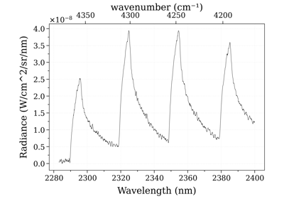
Example #3: non-equilibrium spectrum (Tvib, Trot, x_CO)
Example #3: non-equilibrium spectrum (Tvib, Trot, x_CO)See also
- planck(lambda_, T, eps=1, unit='mW/cm2/sr/nm')[source]
Planck function for blackbody radiation.
\[\epsilon \frac{2h c^2}{{\lambda}^5} \frac{1}{\operatorname{exp}\left(\frac{h c}{\lambda k T}\right)-1}\]- Parameters:
λ (np.array (nm)) – wavelength
T (float (K)) – equilibrium temperature
eps (grey-body emissivity) – default 1
unit (output unit) – default ‘mW/sr/cm2/nm’
- Returns:
np.array – equilibrium radiance
- Return type:
(mW.sr-1.cm-2/nm)
See also
sPlanck(),planck_wn()
- planck_wn(wavenum, T, eps=1, unit='mW/cm2/sr/cm-1')[source]
Planck function for blackbody radiation, wavenumber version.
\[\epsilon 2h c^2 {\nu}^3 \frac{1}{\operatorname{exp}\left(\frac{h c \nu}{k T}\right)-1}\]- Parameters:
wavenum (np.array (cm-1)) – wavenumber
T (float (K)) – equilibrium temperature
eps (grey-body emissivity) – default 1
unit (str) – output unit. Default ‘mW/sr/cm2/cm-1’
- Returns:
np.array – equilibrium radiance
- Return type:
default (mW/sr/cm2/cm-1)
See also
sPlanck(),planck()
- plot_diff(s1: Spectrum, s2: Spectrum, var=None, wunit='default', Iunit='default', resample=True, method='diff', diff_window=0, show_points=False, label1=None, label2=None, figsize=None, title=None, nfig=None, normalize=False, yscale='linear', verbose=True, save=False, show=True, show_residual=False, lw_multiplier=1, diff_scale_multiplier=1, discard_centile=0, plot_medium='vacuum_only', legendargs={'loc': 'best'}, show_ruler=False)[source]
Plot two spectra, and the difference between them.
method=allows you to plot the absolute difference, ratio, or both.If waveranges dont match,
s2is interpolated overs1.- Parameters:
s1, s2 (Spectrum objects)
var (str, or None) – spectral quantity to plot (ex:
'abscoeff'). If None, plot the first one in the Spectrum from'radiance','radiance_noslit','transmittance', etc.wunit (
'default','nm','cm-1','nm_vac') – wavespace unit: wavelength air, wavenumber, wavelength vacuum. If'default', use first spectrum wunitIunit (str) – if
'default', use first spectrum unitmethod (
'distance','diff','ratio', or list of them.) – If'diff', plot difference of the two spectra. If'distance', plot Euclidian distance (note that units are meaningless then) If'ratio', plot ratio of two spectra Default'diff'.Warning
with
'distance', calculation scales as ~N^2 with N the number of points in a spectrum (against ~N with'diff'). This can quickly override all memory.Can also be a list:
method=['diff', 'ratio']
normalize (bool) – Normalize the spectra to be plotted
- Other Parameters:
plot yscale
yscale: ‘linear’, ‘log diff_window: int
If non 0, calculates diff by offsetting s1 by
diff_windownumber of units on either side, and returns the minimum. Kinda compensates for experimental errors on the w axis. Default 0. (look up code to understand…)- show_points: boolean
if
True, make all points appear with ‘o’- label1, label2: str
curve names
- figsize
figure size
- nfig: int, str
figure number of name
- title: str
title
- verbose: boolean
if
True, plot stuff such as rescale ratio in normalize mode. DefaultTrue- save: str
Default is
False. By default won’t save anything, type the path of the destination if you want to save it (format in the name).- show: Bool
Default is
True. Will show the plots. You should switch toFalseif there are more than 20 calls of this function to avoid memory load during execution. IfFalse, you can show the plot(s) withplt.show()- show_residual: bool
if
True, calculates and shows on the graph the residual in L2 norm. Seeget_residual().diff_windowis used in the residual calculation too.normalizehas no effect.- diff_scale_multiplier: float
dilate the diff plot scale. Default
1- discard_centile: int
if not
0, discard the firsts and lasts centile when setting the limits of the diff window. Example:discard_centile=1 # --> discards the smallest 1% and largest 1% discard_centile=10 # --> discards the smallest 10% and largest 10%
Useful to remove spikes in a ratio, for instance. Note that this does not change the values of the residual. It’s just a plot feature. Default
0- plot_medium: bool,
'vacuum_only' if
Trueandwunitare wavelengths, plot the propagation medium in the xaxis label ([air]or[vacuum]). If'vacuum_only', plot only ifwunit=='nm_vac'. Default'vacuum_only'(prevents from inadvertently plotting spectra with different propagation medium on the same graph).- legendargs: dict
format arguments forwarded to the legend
- show_ruler: bool
if
True, add a ruler tool to the Matplotlib toolbar.Warning
still experimental in 0.9.30 ! Try it, feedback welcome !
- Returns:
fig (figure) – fig
[ax0, ax1] (axes) – spectra and difference axis
Examples
Simple use:
from radis import plot_diff
plot_diff(s10, s50)                # s10, s50 are two spectra
Advanced use, plotting the total power in the label, and getting the figure and axes handle to edit them afterwards:
Punit = 'mW/cm2/sr'
fig, axes = plot_diff(s10, s50, 'radiance_noslit', figsize=(18,6),
      label1='brd 10 cm-1, P={0:.2f} {1}'.format(s10.get_power(unit=Punit),Punit),
      label2='brd 50 cm-1, P={0:.2f} {1}'.format(s50.get_power(unit=Punit),Punit)
      )
# modify fig, axes..
See an example in Compare two Spectra, which produces the output below:

If you wish to plot in a logscale, it can be done in the following way:
fig, [ax0, ax1] = plot_diff(s0, s1, normalize=False, verbose=False)
ylim0 = ax0.get_ybound()
ax0.set_yscale("log")
ax0.set_ybound(ylim0)
Performance increase of broadening_methods and LDM optimizations.
Performance increase of broadening_methods and LDM optimizations.
Compare OH(A-X) electronic spectra: RADIS vs Specair
Compare OH(A-X) electronic spectra: RADIS vs Specair
Calculate and Compare Spectra for Multiple Molecules
Calculate and Compare Spectra for Multiple MoleculesSee also
get_diff(),get_ratio(),get_distance(),get_residual(),compare_with()
- plot_slit(w, I=None, wunit='', plot_unit='same', Iunit=None, warnings=True, ls='-', title=None, waveunit=None)[source]
Plot slit, calculate and display FWHM, and calculate effective FWHM. FWHM is calculated from the limits of the range above the half width, while FWHM is the equivalent width of a triangular slit with the same area
- Parameters:
w, I (arrays or (str, None)) – if str, open file directly
waveunit (
'nm','cm-1'or'') – unit of input wplot_unit (
'nm','cm-1'or'same') – change plot unit (and FWHM units)Iunit (str, or None) – give Iunit
warnings (boolean) – if True, test if slit is correctly centered and output a warning if it is not. Default
True
- Returns:
fix, ax – figure and ax
- Return type:
matplotlib objects
Examples
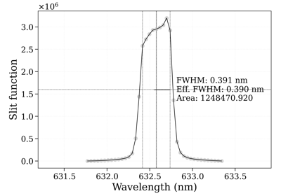
- plot_spec(file, what='radiance', title=True, **kwargs)[source]
Plot a .spec file. Uses the
plot()method internally.- Parameters:
file (str, or Spectrum object) – .spec file to load, or Spectrum object directly
- Other Parameters:
kwargs (dict) – arguments forwarded to
plot()- Returns:
fig – where the Spectrum has been plotted
- Return type:
matplotlib figure
See also
- sPlanck(wavenum_min=None, wavenum_max=None, wavelength_min=None, wavelength_max=None, T=None, eps=1, wstep=0.01, medium='air', **kwargs)[source]
Return a RADIS
Spectrumobject with blackbody radiation.It’s easier to plug in a
SerialSlabs()line-of-sight than the Planck radiance calculated byplanck(). And you don’t need to worry about units as they are handled internally.See
Spectrumdocumentation for more information- Parameters:
wavenum_min / wavenum_max (():math:
cm^{-1})) – minimum / maximum wavenumber to be processed in \(cm^{-1}\).wavelength_min / wavelength_max ((\(nm\))) – minimum / maximum wavelength to be processed in \(nm\).
T (float (K)) – blackbody temperature
eps (float [0-1]) – blackbody emissivity. Default
1
- Other Parameters:
wstep (float (cm-1 or nm)) – wavespace step for calculation
**kwargs (other keyword inputs) – all are forwarded to spectrum conditions. For instance you can add a ‘path_length=1’ after all the other arguments
Examples
Generate Earth blackbody:
s = sPlanck(wavelength_min=3000, wavelength_max=50000,
            T=288, eps=1)
s.plot()
Examples using sPlanck :
References
In wavelength:
\[\epsilon \frac{2h c^2}{{\lambda}^5} \frac{1}{\operatorname{exp}\left(\frac{h c}{\lambda k T}\right)-1}\]In wavenumber:
\[\epsilon 2h c^2 {\nu}^3 \frac{1}{\operatorname{exp}\left(\frac{h c \nu}{k T}\right)-1}\]Additional Reference: - [“Blackbody Radiation and Planck’s Law,” Optics Express] (https://opg.optica.org/oe/fulltext.cfm?uri=oe-14-18-8121&id=97928).
See also

- save(s: Spectrum, path, discard=[], compress=True, add_info=None, add_date=None, if_exists_then='increment', verbose=True, warnings=True)[source]
Save a
Spectrumobject in JSON format. Object can be recovered withload_spec(). If manySpectrumare saved in a same folder you can view their properties with theSpecDatabasestructure.- Parameters:
s (Spectrum) – to save
path (str or file-like object) – If a string: filename to save. No extension needed. If filename already exists then a digit is added. If filename is a directory then a new file is created within this directory.
If a file-like object (e.g.,
io.BytesIO,io.StringIO): writes directly to the object without any file system operations. UseBytesIOwhencompress=True(binary output), useStringIOwhencompress=False(text output). When using file-like objects, theadd_date,add_info, andif_exists_thenparameters are ignored.discard (list of str) – parameters to discard. To save some memory.
compress (boolean) – if
False, save under text format, readable with any editor. ifTrue, saves under binary format. Faster and takes less space. If2, removes all quantities that can be regenerated with s.update(), e.g, transmittance if abscoeff and path length are given, radiance if emisscoeff and abscoeff are given in non-optically thin case, etc. DefaultFalseadd_info (list, or None/False) – append these parameters and their values if they are in conditions. e.g:
add_info = ['Tvib', 'Trot']
add_date (str, or
None/False) – adds date in strftime format to the beginning of the filename. e.g:add_date = '%Y%m%d'
if_exists_then (
'increment','replace','error','ignore') – what to do if file already exists. If'increment'an incremental digit is added. If'replace'file is replaced (!). If'ignore'the Spectrum is not added to the database and no file is created. If'error'(or anything else) an error is raised. Default'increment'.
- Returns:
fout – If path was a string: filename used (may be different from given path as new info or incremental identifiers are added). If path was a file-like object: returns the same object.
- Return type:
str or file-like object
See also
- spectrum_test(**kwargs)[source]
Generate the first example spectrum with
import radis
s = radis.spectrum_test()
s.plot()
- Other Parameters:
kwargs (sent to
calc_spectrum())
- transmittance_spectrum(w, T, wunit='nm', Tunit='', conditions=None, cond_units=None, name=None) Spectrum[source]
Convert
(w, I)into aSpectrumobject that has unit conversion, plotting and slit convolution capabilities.- Parameters:
w (np.array) – wavelength, or wavenumber
T (np.array) – transmittance (no slit)
wunit (
'nm','cm-1','nm_vac') – wavespace unit: wavelength in air ('nm'), wavenumber ('cm-1'), or wavelength in vacuum ('nm_vac'). Default'nm'.Iunit (str) – intensity unit. Default
""(adimensioned)
- Other Parameters:
conditions (dict) – (optional) calculation conditions to be stored with Spectrum
cond_units (dict) – (optional) calculation conditions units
name (str) – (optional) give a name
Examples
# w, T are numpy arrays for wavelength and transmittance
from radis import transmittance_spectrum
s2 = transmittance_spectrum(w, T, wunit='nm')                       # creates 'transmittance_noslit'