


The Spectrum object
RADIS has powerful tools to post-process spectra created by the line-by-line module or by other spectral codes.
At the core of the post-processing is the Spectrum class,
which features methods to:
generate Spectrum objects from text files or python arrays.
rescale a spectrum without redoing the line-by-line calculation.
apply instrumental slit functions.
plot with one line and in whatever unit.
multiply or add constants as simply as with
s=10*sors=s+0.2in Python.store an experimental or a calculated spectrum while retaining the metadata.
combine multiple spectra along the line-of-sight.
manipulate a folder of spectra easily with spectrum Databases.
compute transmittance from absorbance, or whatever missing spectral arrays.
use the line survey tool to identify each line.


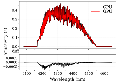
Performance increase of broadening_methods and LDM optimizations.
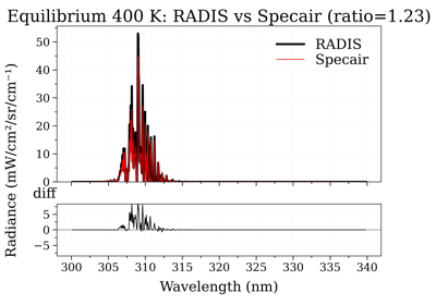
Compare OH(A-X) electronic spectra: RADIS vs Specair


Calculate and Compare Spectra for Multiple Molecules
Example #3: non-equilibrium spectrum (Tvib, Trot, x_CO)
Legacy #2: non-equilibrium CO2 (Tvib_12, Tvib_3, Trot)
Example #7: Database fitting using SpecDatabase.fit_spectrum

Refer to the guide below for an exhaustive list of all features:
For any other question you can use the Q&A forum,
the GitHub issues or the
community chats on Gitter or
Slack . 
![]()
How to generate a Spectrum?
Calculate a Spectrum
Usually a Spectrum object is the output from a line-by-line (LBL) radiation code.
Refer to the LBL documentation for that. Example using the RADIS LBL module with
calc_spectrum():
from radis import calc_spectrum
s = calc_spectrum(...)        # s is a Spectrum object
Or with the SpectrumFactory class, which can
be used to batch-generate multiple spectra using the same line database:
from radis import SpectrumFactory
sf = SpectrumFactory(...)
sf.fetch_databank("hitemp", load_columns='noneq')  # or 'hitran', 'exomol', etc.
s = sf.eq_spectrum(...)
s2 = sf.non_eq_spectrum(...)
Note that the SpectrumFactory class has the
init_database() method that
automatically retrieves a spectrum from a
SpecDatabase if you calculated it already,
or calculates it and stores it if you didn’t. Very useful for spectra that
require long computational times!
Initialize from Python arrays
The standard way to build a Radis Spectrum is from a dictionary of
numpy arrays:
# w, k, I are numpy arrays for wavenumbers, absorption coefficient, and radiance.
from radis import Spectrum
s = Spectrum({"wavenumber":w, "abscoeff":k, "radiance_noslit":I},
             units={"radiance_noslit":"mW/cm2/sr/nm", "abscoeff":"cm-1"})
Or:
s = Spectrum({"abscoeff":(w,k), "radiance_noslit":(w,I)},
             wunit="cm-1"
             units={"radiance_noslit":"mW/cm2/sr/nm", "abscoeff":"cm-1"})
You can also use the from_array()
convenience function:
# w, T are two numpy arrays
from radis import Spectrum
s = Spectrum.from_array(w, T, 'transmittance_noslit',
                           wunit='nm', unit='') # adimensioned
Dimensioned arrays can also be used directly
import astropy.units as u
w = np.linspace(200, 300) * u.nm
I = np.random.rand(len(w)) * u.mW/u.cm**2/u.sr/u.nm
s = Spectrum.from_array(w, I, 'radiance_noslit')
Other convenience functions have been added to handle the usual cases:
calculated_spectrum(),
transmittance_spectrum() and
experimental_spectrum():
# w, T, I are numpy arrays for wavelength, transmittance and radiance
from radis import calculated_spectrum, transmittance_spectrum, experimental_spectrum
s1 = calculated_spectrum(w, I, wunit='nm', Iunit='W/cm2/sr/nm')     # creates 'radiance_noslit'
s2 = transmittance_spectrum(w, T, wunit='nm')                       # creates 'transmittance_noslit'
s3 = experimental_spectrum(w, I, wunit='nm', Iunit='W/cm2/sr/nm')   # creates 'radiance'
Initialize from Specutils
Use from_specutils() to convert
from a specutils specutils.spectra.spectrum1d.Spectrum1D object
from radis import Spectrum
Spectrum.from_specutils(spectrum)
Initialize from a text file
Spectrum objects can also be generated directly from a text file.
From a file, use from_txt()
# 'exp_spectrum.txt' contains a spectrum
from radis import Spectrum
s = Spectrum.from_txt('exp_spectrum.txt', 'radiance',
                           wunit='nm', unit='mW/cm2/sr/nm')
It is, however, recommended to use the RADIS .spec json format to store
and load arrays :
Load from a .spec file
A .spec file contains all the Spectrum spectral arrays as well as the input
conditions used to generate it. To retrieve it use the
load_spec() function:
s = load_spec('my_spectrum.spec')
Sometimes the .spec file may have been generated under a compressed format
where redundant spectral arrays have been removed (for instance, transmittance
if you already know absorbance). Use the update()
method to regenerate missing spectral arrays:
s = load_spec('my_spectrum.spec', binary=True)
s.update()
If many spectra are stored in a folder, it may be time to set up a
SpecDatabase structure to easily see all
Spectrum conditions and get Spectrum that suits specific parameters
Example #3: non-equilibrium spectrum (Tvib, Trot, x_CO)
Load from a HDF5 file
This is the fastest way to read a Spectrum object from disk. It keeps metadata
and units, and you can also load only a part of a very large spectrum.
Use from_hdf5()
Spectrum.from_hdf5("rad_hdf.h5", wmin=2100, wmax=2200, columns=['abscoeff', 'emisscoeff'])
Calculate a test spectrum
You need a spectrum immediatly, to run some tests ? Use spectrum_test()
s = radis.spectrum_test()
s.apply_slit(0.5, 'nm')
s.plot('radiance')
This returns the CO spectrum from the first documentation example
Generate a Blackbody (Planck) function object
In RADIS you can either use the planck() and
planck_wn() functions that generate Planck
radiation arrays for wavelength and wavenumber, respectively.
Or, you can use the sPlanck() function that
returns a Spectrum object, with all
the associated methods (add in a line-of-sight, compare, etc.)
Example:
s = sPlanck(wavelength_min=3000, wavelength_max=50000,
            T=288, eps=1)
s.plot()
Spectral Arrays
A Spectrum object can contain one spectral arrays, such as
'radiance' for emission spectra, or 'transmittance' for absorption spectra.
It can also contain both emission and absorption quantities to be later combined
with other spectra by solving the radiative transfer equation.
Some variables represent quantities that have been convolved with an instrumental slit function, as measured in experimental spectra:
'radiance': the spectral radiance, convolved by the instrument function (typically in :math:'mW/cm^2/sr/nm'). This is sometimes confusingly called spectral intensity.'transmittance': the directional spectral transmittance (:math:0to :math:1), convolved by the instrument function.'emissivity': the directional spectral emissivity (:math:0to :math:1), convolved by the instrument function. The spectral emissivity is the radiance emitted by a surface divided by that emitted by a black body at the same temperature as that surface. This value is only defined under thermal equilibrium.
Other variables represent quantities that have not been convolved (theoretical spectra):
'radiance_noslit': the spectral radiance (typically in \(mW/cm^2/sr/nm\)). This is sometimes confusingly called spectral intensity.'transmittance_noslit': the directional spectral transmittance (\(0\) to \(1\))'emissivity_noslit': spectral emissivity (0to1) i.e. the radiance emitted by a surface divided by that emitted by a black body at the same temperature as that surface. This value is only defined under thermal equilibrium.'emisscoeff': the directional spectral emission density (typically in \(mW/cm^3/sr/nm\)).'absorbance': the directional spectral absorbance (no dimension), also called optical depth.'abscoeff': spectral absorption coefficient (typically in \(cm^{-1}\)), also called opacity. This is sometimes found as the extinction coefficient in the literature (strictly speaking, extinction is absorption + diffusion, the latter being negligible in the infrared).'xsection': absorption cross-section, typically in cm2
Additionally, RADIS may calculate extra quantities such as:
'emisscoeff_continuum': the pseudo-continuum part of the spectral emission density'emisscoeff', that can be generated bySpectrumFactory'abscoeff_continuum'the pseudo-continuum part of the spectral absorption coefficient'abscoeff', that can be generated bySpectrumFactory
See the latest list in the CONVOLUTED_QUANTITIES and
NON_CONVOLUTED_QUANTITIES.
Custom spectral arrays
A Spectrum object is built on top of a dictionary structure, and can handle
spectral arrays with any name.
Custom spectral arrays with arbitrary units can be defined when creating a Spectrum object, for instance:
# w, I are two numpy arrays
s = Spectrum.from_array(w, I, 'irradiance',
                           wunit='nm', unit='w/cm2/nm')
Although not recommended, it is also possible to directly edit the dictionary containing the objects.
For instance, this is done in
CO2 radiative forcing example
to calculate irradiance from radiance (by multiplying by 'pi' and changing the unit):
s._q['irradiance'] = s.get('radiance_noslit')[1]*pi
s.units['irradiance'] = s.units['radiance_noslit'].replace('/sr', '')
The unit conversion methods will properly work with custom units.
Warning
Rescaling or combining spectra with custom quantities may result in errors.
Relations between quantities
Most of the quantities above can be recomputed from one another. In a homogeneous
slab, one requires an emission spectral density, and an absorption spectral density,
to be able to recompute the other quantities (provided that conditions such as path length
are given). Under equilibrium, only one quantity is needed. Missing quantities
can be recomputed automatically with the update()
method.
Units
Default units are stored in the units dictionary
It is strongly advised not to modify the dictionary above. However, spectral arrays
can be retrieved in arbitrary units with the get()
method.
When a spectral unit is convolved with apply_slit(),
a new convolved spectral array is created. The unit of the convolved spectral array may be different,
depending on how the slit function was normalized. Several options are available in RADIS.
Please refer to the documentation of the apply_slit() method.
How to access Spectrum properties?
Get spectral arrays
Spectral Arrays of a Spectrum object can be stored in arbitrary wavespace (wavenumbers, wavelengths in air, or wavelengths in vacuum) and arbitrary units.
Therefore, it is recommended to use the get()
method to retrieve the quantity un the units you want:
w, I = s.get('transmittance_noslit', wunit='cm-1')
_, R = s.get('radiance_noslit', wunit='nm', Iunit='W/cm2/sr/nm',
             medium='air')
Use with return_units to get dimensioned Astropy Quantities
w, R  = s.get('radiance_noslit', return_units=True)
# w, R are astropy quantities
See spectral arrays for the list of spectral arrays.
Get wavelength/wavenumber
Use the get_wavelength() and
get_wavenumber() methods:
w_nm = s.get_wavelength()
w_cm = s.get_wavenumber()
Print Spectrum conditions
Want to know under which calculation conditions was your Spectrum object generated, or under which experimental conditions it was measured? Just print it:
print(s)
(it shows all spectral arrays stored in the object, all keys and
values in the conditions dictionary,
and all atoms/molecules stored in the populations
dictionary)
You can also show the conditions only with
print_conditions():
s.print_conditions()
Get condition
To get a calculation or input condition, use :py:meth`~radis.spectrum.spectrum.Spectrum.get_condition` which can return condition in arbitrary units:
pressure_Pa, _ = s.get_condition("pressure", "Pa", return_unit=True)
Plot spectral arrays
Use plot():
s.plot('radiance_noslit')
You can plot on the same figure as before using the convenient nfig parameter:
s_exp.plot('radiance_noslit', nfig='same')
But for comparing different spectra you may want to use
plot_diff() directly.
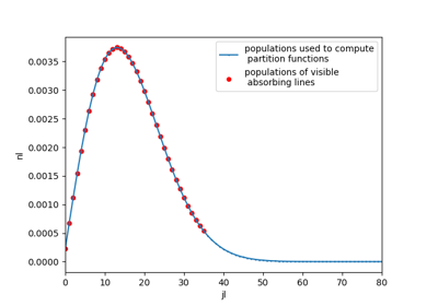
Plot populations
Get or plot populations computed in calculations.
Use get_populations()
or plot_populations():
s.plot_populations('vib', nunit='cm-3')
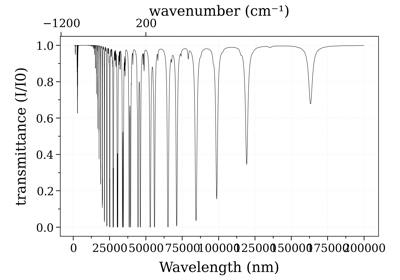
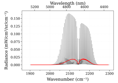
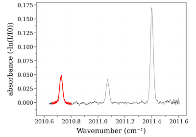
Plot line survey
Use the line_survey() method.
Example of output:
from radis import SpectrumFactory
sf = SpectrumFactory(
                     wavenum_min=2380,
                     wavenum_max=2400,
                     mole_fraction=400e-6,
                     path_length=100,  # cm
                     isotope=[1],
                     )
sf.load_databank('HITRAN-CO2-TEST')
s = sf.eq_spectrum(Tgas=1500)
s.apply_slit(0.5)
s.line_survey(overlay='radiance_noslit', barwidth=0.01)
Know if a spectrum has nan
has_nan() looks over all spectral
quantities. print(s) will also show the number of nans per quantity
s = radis.spectrum_test()
s.has_nan()
How to export ?
Save a Spectrum object
To store use the store() method:
# s is a Spectrum object
s.store('temp_file.spec')
from radis import load_spec
s2 = load_spec('temp_file.spec')
assert s == s2  # compare both
The generated .spec file can be read (and edited) with any text editor. However,
it may take a lot of space. If memory is important, you may use the compress=True
argument which will remove redundant spectral arrays (for instance, transmittance
if you already know absorbance), and store the .spec file under binary format. Use
the update() method to regenerate missing
quantities:
s.store('temp_file.spec', compress=True, if_exists_then='replace')
s2 = load_spec('temp_file.spec')
s2.update()    # regenerate missing quantities
If calculating many spectra, you may want to handle all of them together
in a SpecDatabase. You can add them to the existing
database with the add() method:
db = SpecDatabase(r"path/to/database")     # create or loads database
db.add(s)
Note that if using the RADIS LBL code to generate your spectra, the
SpectrumFactory class has the
init_database() method that
automatically retrieves a spectrum from a database if you calculated it already,
or calculates it and stores it if you didn’t. Very useful for spectra that
requires long computational times!
Export to hdf5
This is the fastest way to dump a Spectrum object on disk (and also, it keeps metadata
and therefore units !). Use to_hdf5()
s.to_hdf5('spec01.h5')
Export to txt
Saving to .txt in general isn’t recommended as you will loose some information (for instance,
the conditions). You better use store() and export
to .spec [a hidden .json] format.
If you really need to export a given spectral arrays to txt file (for use in another software,
for instance), you can use the savetxt() method that
will export a given spectral arrays:
s.savetxt('radiance_W_cm2_sr_um.csv', 'radiance_noslit', wunit='nm', Iunit='W/cm2/sr/µm')
Export to Pandas
Use to_pandas()
s.to_pandas()
This will return a DataFrame with all spectral arrays as columns.
Export to Specutils
Use to_specutils() to convert
to a to specutils specutils.spectra.spectrum1d.Spectrum1D object
s.to_specutils()
How to modify a Spectrum object?
Calculate missing quantities
Some spectral arrays can be inferred from quantities stored in the Spectrum if enough conditions are given. For instance, transmittance can be recomputed from the spectral absorption coefficient if the path length is stored in the conditions.
The update() method can be used to do that.
In the example below, we recompute transmittance from the absorption coefficient
(opacity)
# w, A are numpy arrays for wavenumber and absorption coefficient
s = Spectrum.from_array(w, A, 'abscoeff', wunit='cm-1')
s.update('transmittance_noslit')
All derivable quantities can be computed using .update('all') or simply .update():
s.update()
Update Spectrum conditions
Spectrum conditions are stored in a conditions dictionary
Conditions can be updated a posteriori by modifying the dictionary:
s.conditions['path_length'] = 10 # cm
Rescale Spectrum with new path length
Path length can be changed after the spectra were calculated with the
rescale_path_length() method.
If the spectrum is not optically thin, this requires solving the radiative
transfer equation again, so the emisscoeff and abscoeff (opacity) quantities
will have to be stored in the Spectrum, or any equivalent combination
(radiance_noslit and absorbance, for instance).
Example:
from radis import load_spec
s = load_spec('co_calculation.spec')
s.rescale_path_length(0.5)      # calculate for new path_length
Rescale Spectrum with new mole fraction
Warning
Rescaling mole fractions neglects the changes in collisional broadening
mole fraction can also be changed in post-processing, using the
rescale_mole_fraction() method
that works similarly to the rescale_path_length()
method. However, the broadening coefficients are left unchanged, which is
valid for small mole fraction changes. However, for large mole fraction changes
you will have to recalculate the spectrum from scratch.
>>> s.rescale_mole_fraction(0.02) # calculate for new mole fraction
Apply instrumental slit function
Use apply_slit():
s.apply_slit(1.5) # nm
By default, convoluted spectra are thinner than non-convoluted spectra, to remove
side effects. Use the mode= argument to change this behavior.
Compare OH(A-X) electronic spectra: RADIS vs Specair
Plot the slit function that was applied
Use plot_slit(). You can also
change the unit:
s.apply_slit(0.5, 'cm-1')    # for instance
s.plot_slit('nm')
Multiply, subtract
Sometimes you need to manipulate an experimental spectrum, to account for calibration or remove a baseline. Spectrum operations are done just for that:
Most of these functions are implemented with the standard operators. Ex:
((s_exp - 0.1)*10).plot() # works for a Spectrum s_exp
Note that these operators are purely algebraic and should not be used in place
of the line-of-sight functions, i.e, SerialSlabs() (>)
and MergeSlabs() (//)
Most of these functions will only work if there is only one
spectral arrays
defined in the Spectrum. If there is any ambiguity, use the take()
method. For instance, the following line is a valid RADIS command to plot
the spectral radiance of a spectrum with a low resolution:
(10*(s.apply_slit(10, 'nm')).take('radiance')).plot()
Algebraic operations also work with dimensioned Quantity.
For instance, remove a constant baseline in a given unit:
s -= 0.1 * u.Unit('W/cm2/sr/nm')
The max() function returns a dimensioned
value, therefore it can be used to normalize a spectrum directly :
s /= s.max()
Or below, we calibrate a Spectrum, assuming the spectrum units is in “count”, and that our calibration show we have 94 \(mW/cm2/sr/nm\) per count.
s *= 94 * u.Unit("mW/cm2/sr/nm") / u.Unit("count")
Offset, crop
Use the associated functions: crop(),
offset().
They are also defined as methods of the Spectrum objects (see
crop(), offset()),
so they can be used directly with:
s.offset(3, 'nm')
s.crop(370, 380, 'nm')
By default, using methods that will modify the object in place, using the functions will generate a new Spectrum.
Normalize
Use normalize() directly, if your spectrum
only has one spectral arrays
s.normalize()
s.normalize(normalize_how="max")
s.normalize(normalize_how="area")
You can also normalize only on limited range. Useful for noisy spectra
s.normalize(wrange=(2250, 2500), wunit="cm-1", normalize_how="mean")
This returns a new spectrum and does not modify the Spectrum itself. To do so use:
s.normalize(inplace=True)
Chaining
You can chain the various methods of Spectrum. For instance:
s.normalize().plot()
Or:
s.crop(4120, 4220, 'nm').apply_slit(3, 'nm').take('radiance')
If you want to create a new spectrum, don’t forget to set inplace=False
for the first command that allows it. i.e
s2 = s.crop(4120, 4220, 'nm', inplace=False).apply_slit(3, 'nm').offset(1.5, 'nm')
Remove a baseline
Either use the add_constant() mentioned
above, which is implemented with the - operator:
s2 = s - 0.1
Or remove a linear baseline with:
You could also use the functions available in pyspecutils,
see to_specutils().
Calculate transmittance from radiance with Kirchoff’s law
RADIS can be used to infer spectral arrays from others if they can
be derived. If on top that, equilibrium is assumed, then Kirchoff’s law
is used. See How to ... calculate missing quantities? and the
update() method with argument assume_equilibrium=True.
Example:
s = calculated_spectrum(...)     # defines 'radiance_noslit')
s.update('transmittance_noslit')
s.plot('transmittance_noslit')
You can infer if a Spectrum is at (thermal) equilibrium with the
is_at_equilibrium() method, that
looks up the declared spectrum conditions and ensures Tgas==Tvib==Trot.
It does not imply chemical equilibrium (mole fractions are still arbitrary)
How to handle multiple Spectra?
Build a line-of-sight profile
RADIS allows the combination of Spectra such as:
s_line_of_sight = (s_plasma_CO2 // s_plasma_CO) > (s_room_absorption)
Refer to the line-of-sight module
Compare two Spectra
You can compare two Spectrum objects using the compare_with()
method, or simply the == statement (which is essentially the same thing):
s1 == s2
>>> True/False
s1.compare_with(s2)
>>> True/False
However, compare_with() allows more freedom
regarding what quantities to compare. == will compare everything of two spectra,
including input conditions, units under which spectral quantities are stored,
populations of species if they were saved, etc. In many situations, we may want
to simply compare the spectra themselves, or even a particular quantity like
transmittance_noslit. Use:
s1.compare_with(s2, spectra_only=True)                    # compares all spectral arrays
s1.compare_with(s2, spectra_only='transmittance_noslit')  # compares transmittance only
The aforementioned methods will return a boolean array (True/False). If you
need the difference, or ratio, or distance, between your two spectra, or simply
want to plot the difference, you can use one of the predefined functions
get_diff(), get_ratio(),
get_distance(), get_residual()
or the plot function plot_diff():
from radis.spectrum import plot_diff
s1 = load_spec(temp_file_name)
s2 = load_spec(temp_file_name2)
plot_diff(s1, s2, 'radiance')
These functions usually require that the spectra are calculated on the same spectral
range. When comparing, let’s say, a calculated spectrum with experimental data,
you may want to interpolate: you can have a look at the resample()
method. See Interpolate a Spectrum on another for details.
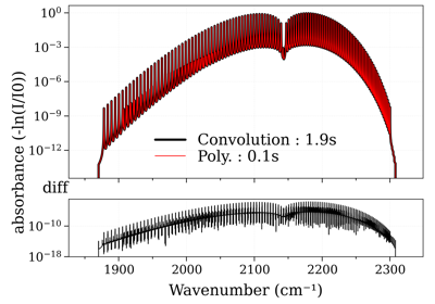
In plot_diff(), you can choose to plot the absolute difference
(method='diff'), or the ratio (method='ratio'), or both:
# Below we compare 2 CO2 spectra s_cdsd and s_hitemp previously calculated with two different line databases.
from radis import plot_diff
plot_diff(s_cdsd, s_hitemp, method=['diff', 'ratio'])

Plot in log scale
If you wish to plot in a logscale, it can be done in the following way:’:
fig, [ax0, ax1] = plot_diff(s_expe, s_test, normalize=False, verbose=False)
ylim0 = ax0.get_ybound()
ax0.set_yscale("log")
ax0.set_ybound(ylim0)
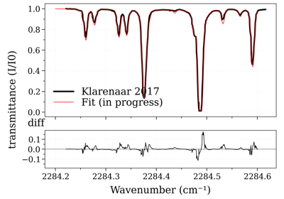
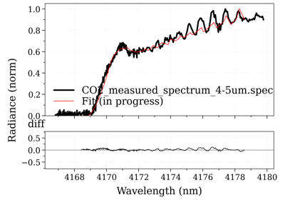
Fit an experimental spectrum
RADIS does not include fitting algorithms. To fit an experimental spectrum, one
should use one of the widely available optimization algorithms from the Python
ecosystem, for instance scipy.optimize.minimize().
The get_residual() and
get_residual_integral() functions can
be used to return a scalar to feed to the minimize()
function.
A simple fitting procedure could be:
from scipy.optimize import minimize
from radis import calc_spectrum, experimental_spectrum

s_exp = experimental_spectrum(...)

def cost_function(T):
    calc_spectrum(Tgas=T,
                  ... # other parameters )
    return get_residual(s_exp, s)

best = minimize(cost_function,
                  800, # initial value
                  bounds=[500, 2000],
                  )
T_best = best.x
Note however that the performances of a fitting procedure can be
vastly improved by not reloading the line database every time. In that
case, it becomes interesting to use the SpectrumFactory
class.
An example of a script that uses the SpectrumFactory,
multiple fitting parameters, and plots the residual and the calculated spectrum
in real-time, can be found in the Fitting examples.
Interpolate a Spectrum on another
Let’s interpolate a calculated spectrum on an experimental spectrum,
using the resample() and, for instance,
the get_wavelength() method:
# let's say we have two objects:
s_exp = load_spec('...')
s_calc = calc_spectrum(...)
# resample:
s_calc.resample(s_exp.get_wavelength(), 'nm')
Energy conservation is ensured and an error is raised if your interpolation
is too bad. If you need to adjust the error threshold, see the parameters
in resample().
Create a database of Spectrum objects
Use the SpecDatabase class. It takes a
folder as an argument, and converts it in a list of
Spectrum objects. Then, you can:
see the properties of all spectra within this folder with
see()select the Spectrum that match a given set of conditions with
get(),get_unique()andget_closest()fit an experimental spectrum against all precomputed spectra in the folder with
fit_spectrum()
See more information about databases below.
Spectrum Database
Spectrum objects can be stored/loaded to/from
.spec JSON files using the store() method
and the load_spec() function.
Example #7: Database fitting using SpecDatabase.fit_spectrum
It is also possible to set up a SpecDatabase
which reads all .spec files in a folder. The SpecDatabase
can then be connected to a SpectrumFactory so that
spectra already in the database are not recomputed, and that new calculated spectra
are stored in the folder
Example:
db = SpecDatabase(r"path/to/database")     # create or loads database

db.update()  # in case something changed
db.see(['Tvib', 'Trot'])   # nice print in console

s = db.get('Tvib==3000')[0]  # get a Spectrum back
db.add(s)  # update database (and raise error because duplicate!)
A SpecDatabase can also be used to
compare the physical and computation parameters of all spectra in a folder.
Indeed, whenever the database is loaded, a summary .csv file
is generated that contains all conditions and can be read, for instance,
with Excel.
Example:
from radis import SpecDatabase
SpecDatabase(r".")     # this generates a .csv file in the current folder
The examples below show some actions that can be performed on a database:
Iterate over all Spectra in a database
Both methods below are equivalent. Directly iterating over the database:
db = SpecDatabase('.')
for s in db:
    print(s.name)
Or using the get() method with
no filtering condition:
db = SpecDatabase('.')
for s in db.get():
    print(s.name)
You can also use dictionary-like methods: keys(),
values() and items()
where Spectrum are returned under a {path:Spectrum} dictionary.
Filter spectra that match certain conditions
If you want to get Spectra in your database that match certain conditions
(e.g: a particular temperature), you may want to have a look at the
get(),
get_unique() and
get_closest() methods
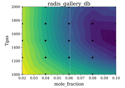
Fit an experimental spectrum against precomputed spectra
The fit_spectrum() method
of SpecDatabase can be used to
return the spectrum of the database that matches the best an experimental
spectrum:
s_exp = experimental_spectrum(...)
db = SpecDatabase('...')
db.fit_spectrum(s_exp)
By default fit_spectrum() uses
the get_residual() function. You can use
an customized function too (below: to get the transmittance):
from radis import get_residual
db.fit_spectrum(s_exp, get_residual=lambda s_exp, s: get_residual(s_exp, s, var='transmittance'))
You don’t necessarily need to precompute spectra to fit an experimental spectrum. You can find an example of multi temperature fitting script in the Fitting examples, which shows the evolution of the spectra in real-time. You can get inspiration from there!
Updating a database
Update all spectra in current folder with a new condition (‘author’), making
use of the items() method:
from radis import SpecDatabase
db = SpecDatabase('.')
for path, s in db.items():
    s.conditions['author'] = 'me'
    s.store(path, if_exists_then='replace')
You may also be interested in the map()
method.
When not to use a Database
If you simply want to store and reload one Spectrum
object, no need to use a database: you better use the store()
method and load_spec() function.
Databases prove useful only when you want to filter precomputed Spectra based on certain conditions.