Example #3: non-equilibrium spectrum (Tvib, Trot, x_CO)

With the new fitting module introduced in fit_spectrum() function, and in the example of Tgas fitting using new fitting module, we can see its 1-temperature fitting performance for equilibrium condition.

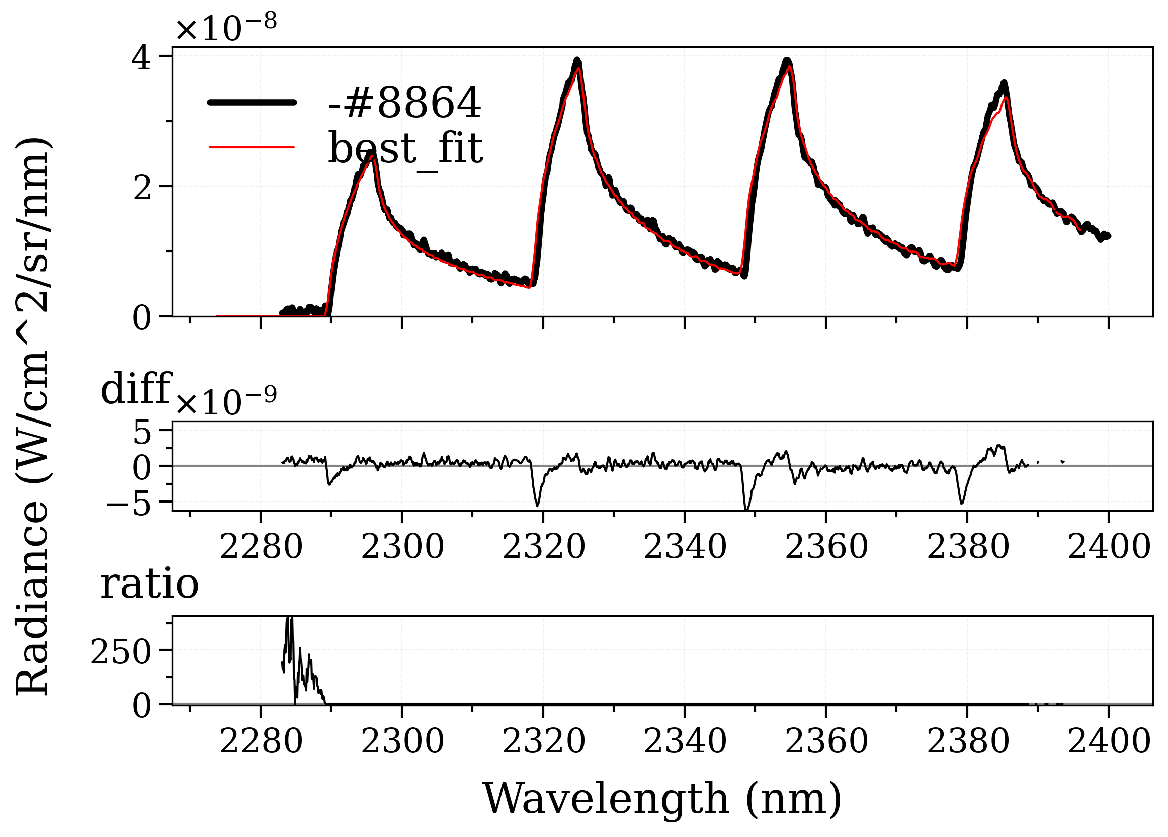
This example features how new fitting module can fit non-equilibrium spectrum, with multiple fit parameters, such as vibrational/rotational temperatures, or mole fraction, etc.

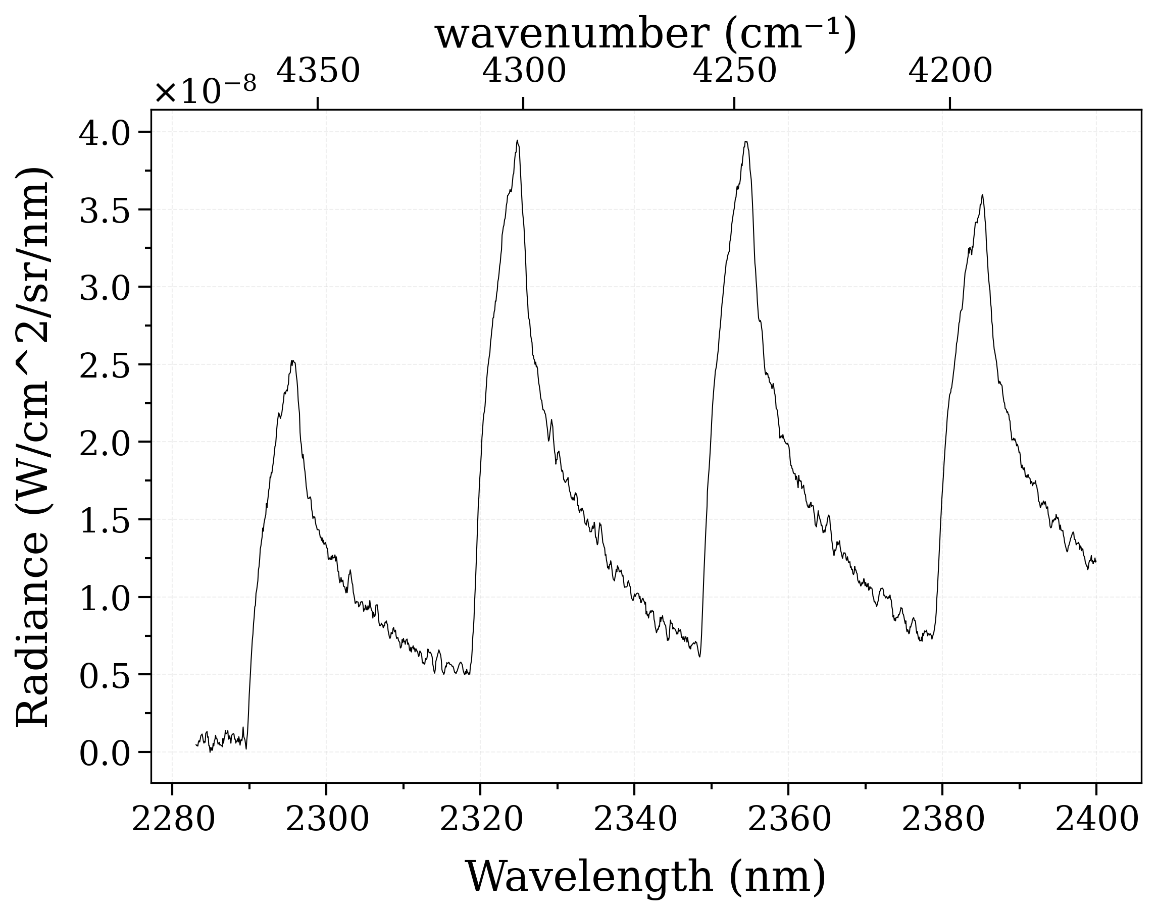
This is a real fitting case introduced Grimaldi’s thesis: https://doi.org/10.2514/1.T6768 . This case features CO molecule emitting on a wide range of spectrum. This case also includes a user-defined trapezoid slit function, which is accounted by the distortion (dispersion) of the slit, as a result of the influences from experimental parameters and spectrometer dispersion parameters during the experiment.

• 
• 

======================= COMMENCE FITTING PROCESS =======================

Successfully retrieved the experimental data in 0.0010330677032470703s.

Acquired spectral quantity 'radiance' from the spectrum.
NaN values successfully purged.Number of data points left: 1479 points.
Successfully refined the experimental data in 0.00039505958557128906s.
/home/docs/checkouts/readthedocs.org/user_builds/radis/checkouts/latest/radis/db/molparam.py:252: FutureWarning:

The 'delim_whitespace' keyword in pd.read_csv is deprecated and will be removed in a future version. Use ``sep='\s+'`` instead


Commence fitting process for non-LTE spectrum!
/home/docs/checkouts/readthedocs.org/user_builds/radis/checkouts/latest/radis/misc/warning.py:427: PerformanceWarning:

'gu' was recomputed although 'gp' already in DataFrame. All values are equal

[[Fit Statistics]]
    # fitting method   = L-BFGS-B
    # function evals   = 92
    # data points      = 1
    # variables        = 3
    chi-square         = 1.0967e-21
    reduced chi-square = 1.0967e-21
    Akaike info crit   = -42.2619749
    Bayesian info crit = -48.2619749
##  Warning: uncertainties could not be estimated:
    this fitting method does not natively calculate uncertainties
    and numdifftools is not installed for lmfit to do this. Use
    `pip install numdifftools` for lmfit to estimate uncertainties
    with this fitting method.
[[Variables]]
    Tvib:           4193.70640 (init = 6000)
    Trot:           4029.50286 (init = 4000)
    mole_fraction:  0.07210218 (init = 0.05)

Successfully finished the fitting process in 8.617957353591919s.
/home/docs/checkouts/readthedocs.org/user_builds/radis/checkouts/latest/radis/misc/curve.py:241: UserWarning:

Presence of NaN in curve_divide!
Think about interpolation=2


======================== END OF FITTING PROCESS ========================


Residual history:

[1.2731069613595358e-10, 1.273106981174117e-10, 1.2731069426158152e-10, 1.2731070017060423e-10, 3.884615937110996e-10, 3.8846159304666323e-10, 3.8846159413208926e-10, 3.884615910840761e-10, 9.031556775802106e-11, 9.031556770154134e-11, 9.03155683995552e-11, 9.031556598187334e-11, 8.557352690375277e-11, 8.55735275489347e-11, 8.557352685839632e-11, 8.557352689776171e-11, 8.454418034621256e-11, 8.454418096961944e-11, 8.454418033305902e-11, 8.454418025390262e-11, 8.051804532456135e-11, 8.051804581217556e-11, 8.05180454785717e-11, 8.051804482369926e-11, 7.564923946247372e-11, 7.56492382627784e-11, 7.564924065877926e-11, 7.564923663861085e-11, 6.446529598361958e-11, 6.44652959563408e-11, 6.446529651558233e-11, 6.446529467077107e-11, 4.128674962809009e-11, 4.12867477220696e-11, 4.1286750611256466e-11, 4.1286747782614464e-11, 4.0435316151769e-11, 4.0435318759511845e-11, 4.043531491796889e-11, 4.043531768458092e-11, 3.605101293549589e-11, 3.605101325520536e-11, 3.605101284203708e-11, 3.6051012764048195e-11, 3.546001725098928e-11, 3.54600160067941e-11, 3.546001745781015e-11, 3.546001664222057e-11, 3.441863053628808e-11, 3.4418630349973597e-11, 3.4418630491064437e-11, 3.4418630265340955e-11, 3.40108143294477e-11, 3.4010814189860064e-11, 3.4010814226497004e-11, 3.401081417965744e-11, 3.343695175796535e-11, 3.343695172687317e-11, 3.343695165155156e-11, 3.343695174141517e-11, 3.315438911578275e-11, 3.3154389121495445e-11, 3.3154389068345065e-11, 3.3154389137110534e-11, 3.3117363908755194e-11, 3.31173639135497e-11, 3.311736390055919e-11, 3.311736391445633e-11, 3.3116571998635484e-11, 3.3116571996638406e-11, 3.31165719986872e-11, 3.3116571997787036e-11, 3.3116570435176885e-11, 3.311657043687362e-11, 3.311657043525792e-11, 3.311657043578823e-11, 3.311656608851647e-11, 3.311656608836644e-11, 3.3116566088295416e-11, 3.311656608857933e-11, 3.311656740914238e-11, 3.311656740889514e-11, 3.3116567409583644e-11, 3.3116567408841747e-11, 3.311656614525506e-11, 3.3116566145123655e-11, 3.311656614526467e-11, 3.311656614506565e-11, 3.3116566081363785e-11, 3.311656608122754e-11, 3.3116566081536285e-11, 3.3116566081090344e-11, 3.3116566081363785e-11]

Fitted values history:

[6000.0, 4000.0, 0.05]
[6000.00002, 4000.0, 0.05]
[6000.0, 4000.000024494898, 0.05]
[6000.0, 4000.0, 0.0500000005]
[5086.091543029117, 4956.218314232288, 0.01315565337609418]
[5086.0915673324025, 4956.218314232288, 0.01315565337609418]
[5086.091543029117, 4956.218338812494, 0.01315565337609418]
[5086.091543029117, 4956.218314232288, 0.013155653714102183]
[5841.32412311191, 4180.011778692965, 0.042174420475386165]
[5841.324144208946, 4180.011778692965, 0.042174420475386165]
[5841.32412311191, 4180.011803487335, 0.042174420475386165]
[5841.32412311191, 4180.011778692965, 0.042174420969224226]
[5854.010651013399, 4135.4895548469085, 0.0445008109929573]
[5854.010672029239, 4135.4895548469085, 0.0445008109929573]
[5854.010651013399, 4135.489579579746, 0.0445008109929573]
[5854.010651013399, 4135.4895548469085, 0.04450081148992399]
[5820.374792038889, 4135.405575013761, 0.04468975287277822]
[5820.374813267668, 4135.405575013761, 0.04468975287277822]
[5820.374792038889, 4135.405599746475, 0.04468975287277822]
[5820.374792038889, 4135.405575013761, 0.04468975336995035]
[5682.56985616577, 4135.069659885674, 0.045446260324148474]
[5682.569878191956, 4135.069659885674, 0.045446260324148474]
[5682.56985616577, 4135.069684617892, 0.045446260324148474]
[5682.56985616577, 4135.069659885674, 0.0454462608220705]
[5089.254134146485, 4133.726066753766, 0.04848106481406099]
[5089.2541584421215, 4133.726066753766, 0.04848106481406099]
[5089.254134146485, 4133.726091483997, 0.04848106481406099]
[5089.254134146485, 4133.726066753766, 0.04848106531383022]
[5156.647156430003, 4090.5780393293185, 0.05028843300338301]
[5156.6471805522215, 4090.5780393293185, 0.05028843300338301]
[5156.647156430003, 4090.5780639917875, 0.05028843300338301]
[5156.647156430003, 4090.5780393293185, 0.05028843350337469]
[4369.438281197388, 3911.423034882001, 0.06277817077420146]
[4369.4383061632725, 3911.423034882001, 0.06277817077420146]
[4369.438281197388, 3911.423059179279, 0.06277817077420146]
[4369.438281197388, 3911.423034882001, 0.0627781712575976]
[4383.82699664511, 3810.6412353794526, 0.0662198270331835]
[4383.827021618103, 3810.6412353794526, 0.0662198270331835]
[4383.82699664511, 3810.641259410234, 0.0662198270331835]
[4383.82699664511, 3810.6412353794526, 0.0662198275061441]
[4376.791308135788, 3859.778263298098, 0.06454646280475469]
[4376.79133310541, 3859.778263298098, 0.06454646280475469]
[4376.791308135788, 3859.7782874644304, 0.06454646280475469]
[4376.791308135788, 3859.778263298098, 0.06454646328312698]
[4098.612733420273, 3757.9551695388845, 0.07033304654720018]
[4098.6127580959455, 3757.9551695388845, 0.07033304654720018]
[4098.612733420273, 3757.9551934122364, 0.07033304654720018]
[4098.612733420273, 3757.9551695388845, 0.07033304700398978]
[4240.191510160168, 3809.772858655761, 0.06741274799559943]
[4240.191535024801, 3809.772858655761, 0.06741274799559943]
[4240.191510160168, 3809.7728826840494, 0.06741274799559943]
[4240.191510160168, 3809.772858655761, 0.06741274846429936]
[4200.317473686526, 3818.5163353058215, 0.0688420406890221]
[4200.317498506257, 3818.5163353058215, 0.0688420406890221]
[4200.317473686526, 3818.516359359054, 0.0688420406890221]
[4200.317473686526, 3818.5163353058215, 0.06884204115216112]
[4177.856716471433, 3892.450637218859, 0.07070627776304306]
[4177.856741263013, 3892.450637218859, 0.07070627776304306]
[4177.856716471433, 3892.450661469392, 0.07070627776304306]
[4177.856716471433, 3892.450637218859, 0.07070627821815294]
[4179.94372948883, 3984.957656094384, 0.07195785889100091]
[4179.943754283111, 3984.957656094384, 0.07195785889100091]
[4179.94372948883, 3984.9576805580946, 0.07195785889100091]
[4179.94372948883, 3984.957656094384, 0.07195785934020603]
[4191.6302788453795, 4023.223093725125, 0.07209044106978527]
[4191.630303654467, 4023.223093725125, 0.07209044106978527]
[4191.6302788453795, 4023.223118266282, 0.07209044106978527]
[4191.6302788453795, 4023.223093725125, 0.07209044151833988]
[4193.502403178178, 4029.0408790427264, 0.07210120295507057]
[4193.502427989584, 4029.0408790427264, 0.07210120295507057]
[4193.502403178178, 4029.0409035951143, 0.07210120295507057]
[4193.502403178178, 4029.0408790427264, 0.07210120340357216]
[4193.888458465184, 4029.9124440612527, 0.0721031409260303]
[4193.888483277069, 4029.9124440612527, 0.0721031409260303]
[4193.888458465184, 4029.912468615311, 0.0721031409260303]
[4193.888458465184, 4029.9124440612527, 0.07210314137452235]
[4193.698363868077, 4029.4832779306794, 0.07210218667405076]
[4193.698388679726, 4029.4832779306794, 0.07210218667405076]
[4193.698363868077, 4029.4833024839154, 0.07210218667405076]
[4193.698363868077, 4029.4832779306794, 0.0721021871225475]
[4193.805933927724, 4029.7452415913413, 0.07210215341497815]
[4193.8059587395055, 4029.7452415913413, 0.07210215341497815]
[4193.805933927724, 4029.7452661450793, 0.07210215341497815]
[4193.805933927724, 4029.7452415913413, 0.07210215386347506]
[4193.727769089985, 4029.554887608774, 0.07210217758237426]
[4193.727793901669, 4029.554887608774, 0.07210217758237426]
[4193.727769089985, 4029.554912162148, 0.07210217758237426]
[4193.727769089985, 4029.554887608774, 0.07210217803087106]
[4193.7064037765995, 4029.502857255745, 0.07210218418822413]
[4193.706428588259, 4029.502857255745, 0.07210218418822413]
[4193.7064037765995, 4029.5028818090186, 0.07210218418822413]
[4193.7064037765995, 4029.502857255745, 0.0721021846367209]
[4193.7064037765995, 4029.502857255745, 0.07210218418822413]

Total fitting time:
8.617957353591919 s

import astropy.units as u
import numpy as np

from radis import load_spec
from radis.test.utils import getTestFile
from radis.tools.new_fitting import fit_spectrum

# The following function and parameters reproduce the slit function in Dr. Corenti Grimaldi's thesis.


def slit_dispersion(w):
    phi = -6.33
    f = 750
    gr = 300
    m = 1
    phi *= -2 * np.pi / 360
    d = 1e-3 / gr
    disp = (
        w
        / (2 * f)
        * (-np.tan(phi) + np.sqrt((2 * d / m / (w * 1e-9) * np.cos(phi)) ** 2 - 1))
    )
    return disp  # nm/mm


slit = 1500  # µm
pitch = 20  # µm
top_slit_um = slit - pitch  # µm
base_slit_um = slit + pitch  # µm
center_slit = 5090
dispersion = slit_dispersion(center_slit)
top_slit_nm = top_slit_um * 1e-3 * dispersion
base_slit_nm = base_slit_um * 1e-3 * dispersion * 1.33


# -------------------- Step 1. Load experimental spectrum -------------------- #


specName = (
    "Corentin_0_100cm_DownSampled_20cm_10pctCO2_1-wc-gw450-gr300-sl1500-acc5000-.spec"
)
s_experimental = load_spec(getTestFile(specName)).offset(-0.6, "nm")


# -------------------- Step 2. Fill ground-truths and data -------------------- #


# Experimental conditions which will be used for spectrum modeling. Basically, these are known ground-truths.
experimental_conditions = {
    "molecule": "CO",  # Molecule ID
    "isotope": "1,2,3",  # Isotope ID, can have multiple at once
    "wmin": 2270
    * u.nm,  # Starting wavelength/wavenumber to be cropped out from the original experimental spectrum.
    "wmax": 2400 * u.nm,  # Ending wavelength/wavenumber for the cropping range.
    "pressure": 1.01325
    * u.bar,  # Total pressure of gas, in "bar" unit by default, but you can also use Astropy units.
    "path_length": 1
    / 195
    * u.cm,  # Experimental path length, in "cm" unit by default, but you can also use Astropy units.
    "slit": {  # Experimental slit. In simple form: "[value] [unit]", i.e. "-0.2 nm". In complex form: a dict with parameters of apply_slit()
        "slit_function": (top_slit_nm, base_slit_nm),
        "unit": "nm",
        "shape": "trapezoidal",
        "center_wavespace": center_slit,
        "slit_dispersion": slit_dispersion,
        "inplace": False,
    },
    "cutoff": 0,  # (RADIS native) Discard linestrengths that are lower that this to reduce calculation time, in cm-1.
    "databank": "hitemp",  # Databank used for calculation. Must be stated.
}

# List of parameters to be fitted, accompanied by its initial value
fit_parameters = {
    "Tvib": 6000,  # Vibrational temperature, in K.
    "Trot": 4000,  # Rotational temperature, in K.
    "mole_fraction": 0.05,  # Species mole fraction, from 0 to 1.
}

# List of bounding ranges applied for those fit parameters above.
# You can skip this step and let it use default bounding ranges, but this is not recommended.
# Bounding range must be at format [<lower bound>, <upper bound>].
bounding_ranges = {
    "Tvib": [2000, 7000],
    "Trot": [2000, 7000],
    "mole_fraction": [0, 0.1],
}

# Fitting pipeline setups.
fit_properties = {
    "method": "lbfgsb",  # Preferred fitting method. By default, "leastsq".
    "fit_var": "radiance",  # Spectral quantity to be extracted for fitting process, such as "radiance", "absorbance", etc.
    "normalize": False,  # Either applying normalization on both spectra or not.
    "max_loop": 300,  # Max number of loops allowed. By default, 200.
    "tol": 1e-20,  # Fitting tolerance, only applicable for "lbfgsb" method.
}

"""

For the fitting method, you can try one among 17 different fitting methods and algorithms of LMFIT,
introduced in `LMFIT method list <https://lmfit.github.io/lmfit-py/fitting.html#choosing-different-fitting-methods>`.

You can see the benchmark result of these algorithms here:
`RADIS Newfitting Algorithm Benchmark <https://github.com/radis/radis-benchmark/blob/master/manual_benchmarks/plot_newfitting_comparison_algorithm.py>`.

"""


# -------------------- Step 3. Run the fitting and retrieve results -------------------- #


# Conduct the fitting process!
s_best, result, log = fit_spectrum(
    s_exp=s_experimental,  # Experimental spectrum.
    fit_params=fit_parameters,  # Fit parameters.
    bounds=bounding_ranges,  # Bounding ranges for those fit parameters.
    model=experimental_conditions,  # Experimental ground-truths conditions.
    pipeline=fit_properties,  # # Fitting pipeline references.
)


# Now investigate the result logs for additional information about what's going on during the fitting process

print("\nResidual history: \n")
print(log["residual"])

print("\nFitted values history: \n")
for fit_val in log["fit_vals"]:
    print(fit_val)

print("\nTotal fitting time: ")
print(log["time_fitting"], end=" s\n")