See populations of computed levels

Spectrum methods gives you access to the populations of levels used in a nonequilibrium spectrum :

• get_populations() provides the populations

of all levels of the molecule, used to compute the nonequilibrium partition function

• lines returns all informations

of the visible lines, in particular the populations of the upper and lower levels of absorbing/emitting lines in the spectrum.

from astropy import units as u

We first compute a noneq CO spectrum. Notice the keys export_lines=True and export_populations=True

from radis import calc_spectrum

s = calc_spectrum(
    1900 / u.cm,
    2300 / u.cm,
    molecule="CO",
    isotope="1",
    pressure=1.01325 * u.bar,
    Tvib=3000 * u.K,
    Trot=1000 * u.K,
    mole_fraction=0.1,
    path_length=1 * u.cm,
    databank="hitran",  # or 'hitemp', 'geisa', 'exomol'
    export_lines=True,
    export_populations="rovib",
)

/home/docs/checkouts/readthedocs.org/user_builds/radis/checkouts/latest/radis/io/hitran.py:192: AccuracyWarning: All columns are not downloaded currently, please use cache = 'regen' and extra_params='all' to download all columns.
  warnings.warn(
--------------------------------------------------------------------------------
CO - HITRAN - Downloading database
--------------------------------------------------------------------------------

Download:
- All files already downloaded.

Caching to HDF5/H5 format:
- All files already cached.
0.06s - Loaded database
/home/docs/checkouts/readthedocs.org/user_builds/radis/checkouts/latest/radis/misc/warning.py:434: HighTemperatureWarning: HITRAN is valid for low temperatures (typically < 700 K). For higher temperatures you may need HITEMP or CDSD. See the 'databank=' parameter
  warnings.warn(WarningType(message))
Calculating Non-Equilibrium Spectrum
Physical Conditions
----------------------------------------
   Tgas                 1000.0 K
   Trot                 1000.0 K
   Tvib                 3000.0 K
   isotope              1
   medium               air
   mole_fraction        0.1
   path_length          1.0 cm
   pressure             1.01325 bar
   rot_distribution     boltzmann
   self_absorption      True
   species              CO
   state                X
   vib_distribution     boltzmann
   wavenum_max          2300.0000 cm-1
   wavenum_min          1900.0000 cm-1
Computation Parameters
----------------------------------------
   Tref                 296 K
   add_at_used
   broadening_method    voigt_poly
   cutoff               1e-27 cm-1/(#.cm-2)
   dbformat             hitran
   dbpath               /home/docs/.radisdb/hitran/CO.h5
   diluent              air
   folding_thresh       1e-06
   include_neighbouring_lines  True
   isatom               False
   isneutral            None
   lbfunc               None
   memory_mapping_engine  auto
   neighbour_lines      0 cm-1
   optimization         simple
   parsum_mode          full summation
   pfsource             default
   potential_lowering   None
   pseudo_continuum_threshold  0
   sparse_ldm           auto
   truncation           50 cm-1
   waveunit             cm-1
   wstep                0.01 cm-1
   zero_padding         -1
----------------------------------------
Fetching Evib & Erot.
/home/docs/checkouts/readthedocs.org/user_builds/radis/checkouts/latest/radis/misc/warning.py:434: NegativeEnergiesWarning: There are negative rotational energies in the database
  warnings.warn(WarningType(message))
/home/docs/checkouts/readthedocs.org/user_builds/radis/checkouts/latest/radis/misc/warning.py:434: PerformanceWarning: 'gu' was recomputed although 'gp' already in DataFrame. All values are equal
  warnings.warn(WarningType(message))
... sorting lines by vibrational bands
... lines sorted in 0.0s
0.10s - Spectrum calculated

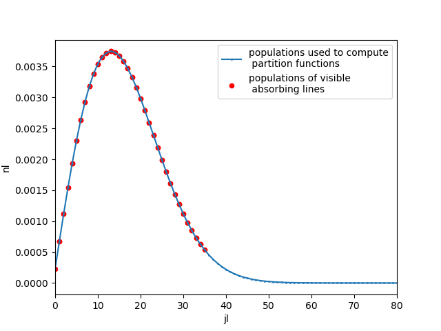
Below we plot the populations We could also have used plot_populations() directly

pops = s.get_populations("CO")["rovib"]

/home/docs/checkouts/readthedocs.org/user_builds/radis/checkouts/latest/radis/spectrum/spectrum.py:2723: UserWarning: Populations valid for partition function calculation but sometimes NOT for spectra calculations, e.g. CO2.
                         See help on how to use 's.lines.query' instead, for instance in https://github.com/radis/radis/issues/508.
                         Turn off warning with 'show_warning=False'

  warn(

Plot populations : Here we plot population fraction vs rotational number of the 2nd vibrational level v==2, for all levels as well as for levels of lines visible in the spectrum

import matplotlib.pyplot as plt

pops.query("v==2").plot(
    "j",
    "n",
    label="populations used to compute\n partition functions",
    style=".-",
    markersize=2,
)
s.lines.query("vl==2").plot(
    "jl",
    "nl",
    ax=plt.gca(),
    label="populations of visible\n absorbing lines",
    kind="scatter",
    color="r",
)
plt.xlim((0, 80))
plt.legend()

<matplotlib.legend.Legend object at 0x73c58f50ea50>

Print all levels information

print(f"{len(pops)} levels ")
print(pops)
print(pops.columns)

7766 levels
       v   j             E  ...             n        Qrot      nrot
0      0   0      0.000000  ...  1.754208e-03  362.691791  0.002757
1      0   1      3.845033  ...  5.233590e-03  362.691791  0.008226
2      0   2     11.534953  ...  8.626674e-03  362.691791  0.013559
3      0   3     23.069466  ...  1.187857e-02  362.691791  0.018670
4      0   4     38.448131  ...  1.493823e-02  362.691791  0.023479
...   ..  ..           ...  ...           ...         ...       ...
7761  48  38  89299.135499  ...  2.237048e-21  360.424333  0.003612
7762  48  39  89447.643402  ...  1.853601e-21  360.424333  0.002993
7763  48  40  89599.882150  ...  1.526677e-21  360.424333  0.002465
7764  48  41  89755.845909  ...  1.249931e-21  360.424333  0.002018
7765  48  42  89915.528699  ...  1.017299e-21  360.424333  0.001643

[7766 rows x 13 columns]
Index(['v', 'j', 'E', 'Evib', 'viblvl', 'gj', 'gvib', 'grot', 'Erot', 'nvib',
       'n', 'Qrot', 'nrot'],
      dtype='str')

Print visible lines information :

print(f"{len(s.lines)} visible lines in the spectrum")
print(s.lines)
print(s.lines.columns)

274 visible lines in the spectrum
             wav           int      A  ...  hwhm_gauss  hwhm_voigt     shiftwav
0    1900.341948  3.611000e-29  12.70  ...    0.004067    0.016713  1900.339087
1    1902.414094  2.342000e-31  25.42  ...    0.004072    0.017474  1902.411257
2    1905.778626  9.225000e-29  12.80  ...    0.004079    0.016872  1905.775770
3    1907.676322  5.419000e-31  25.62  ...    0.004083    0.017672  1907.673489
4    1911.187693  2.314000e-28  12.90  ...    0.004091    0.017028  1911.184842
..           ...           ...    ...  ...         ...         ...          ...
269  2291.548184  1.147000e-28  22.14  ...    0.004905    0.017153  2291.544414
270  2293.336772  4.506000e-29  22.21  ...    0.004909    0.017008  2293.332974
271  2295.082654  1.738000e-29  22.28  ...    0.004912    0.016901  2295.078829
272  2296.785684  6.582000e-30  22.35  ...    0.004916    0.016752  2296.781832
273  2298.445721  2.449000e-30  22.42  ...    0.004919    0.016609  2298.441844

[274 rows x 47 columns]
Index(['wav', 'int', 'A', 'airbrd', 'selbrd', 'El', 'Tdpair', 'Pshft',
       'line_mixing_flag', 'gp', 'gpp', 'branch', 'jl', 'vu', 'vl', 'ju', 'Eu',
       'Evibl', 'Evibu', 'Erotu', 'Erotl', 'gju', 'gjl', 'grotu', 'grotl',
       'gvibu', 'gvibl', 'gu', 'gl', 'viblvl_l', 'viblvl_u', 'band', 'Qrotl',
       'Qrotu', 'nu_vib', 'nl_vib', 'nu_rot', 'nl_rot', 'nu', 'nl', 'S0', 'S',
       'Ei', 'hwhm_lorentz', 'hwhm_gauss', 'hwhm_voigt', 'shiftwav'],
      dtype='str')

We can also look at unique levels; for instance sorting by quantum numbers v, J of the lower level : vl, jl

print(
    len(s.lines.groupby(["vl", "jl"])),
    " visible absorbing levels (i.e. unique 'vl', 'jl' ",
)

141  visible absorbing levels (i.e. unique 'vl', 'jl'

line_survey() is also a convenient way to explore populations and other line parameters, for instance

s.line_survey(overlay="absorbance", barwidth=0.001, lineinfo="all")