Chain Editing and Lineshape Fitting a Spectrum

RADIS includes a powerful chaining syntax to edit (crop/offset/multiply/etc) calculated and experimental spectra. Some examples are given below.

We also do some lineshape fitting using the specutils specutils.fitting.fit_lines() routine and some astropy models, among astropy.modeling.functional_models.Gaussian1D, astropy.modeling.functional_models.Lorentz1D or astropy.modeling.functional_models.Voigt1D

See more loading and post-processing functions on the Spectrum page.

from radis import Spectrum
from radis.test.utils import getTestFile

s = Spectrum.from_mat(
    getTestFile("trimmed_1857_VoigtCO_Minesi.mat"),
    "absorbance",
    wunit="cm-1",
    unit="",
    index=10,
)

# Plot default Spectrum:
s.plot(
    nfig=1,  # nfig=1 and show=False to plot on the same figure after
    show=False,  # needed when using `inline` ploting (e.g. default in Spyder)
)

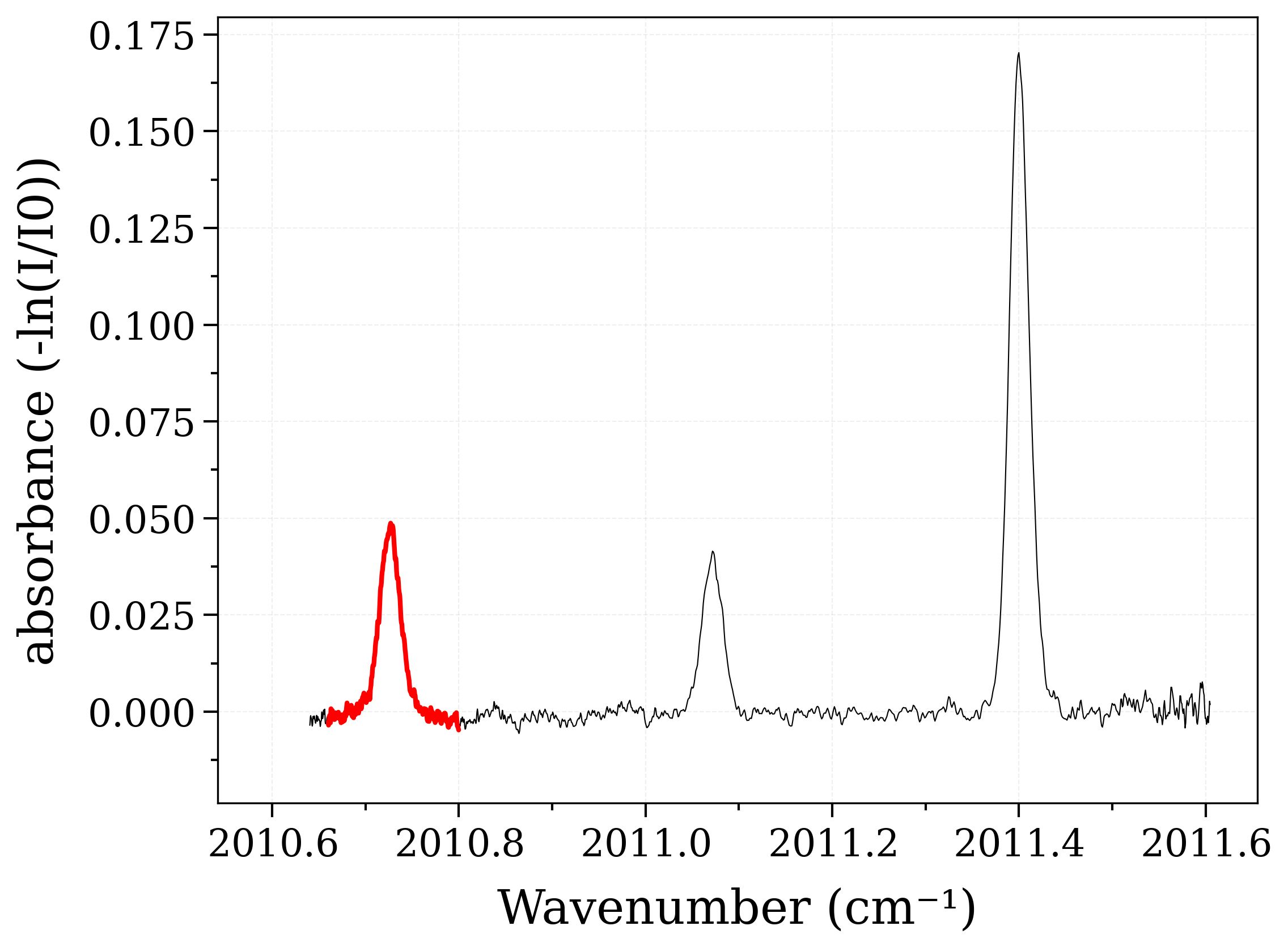
# Now crop to the range we want to study
s.crop(2010.66, 2010.80).plot(
    nfig=1,
    show=True,  # show = True is default
    color="r",
    lw=2,  # plot accepts matlplotlib args
)

/home/docs/checkouts/readthedocs.org/user_builds/radis/checkouts/latest/radis/spectrum/spectrum.py:4921: UserWarning:

Wavespace is not evenly spaced (0.000%) for absorbance. This may create problems if later convolving with slit function (`s.apply_slit()`). You can use `s.resample_even()`


<matplotlib.lines.Line2D object at 0x7fbdf3f2bf70>

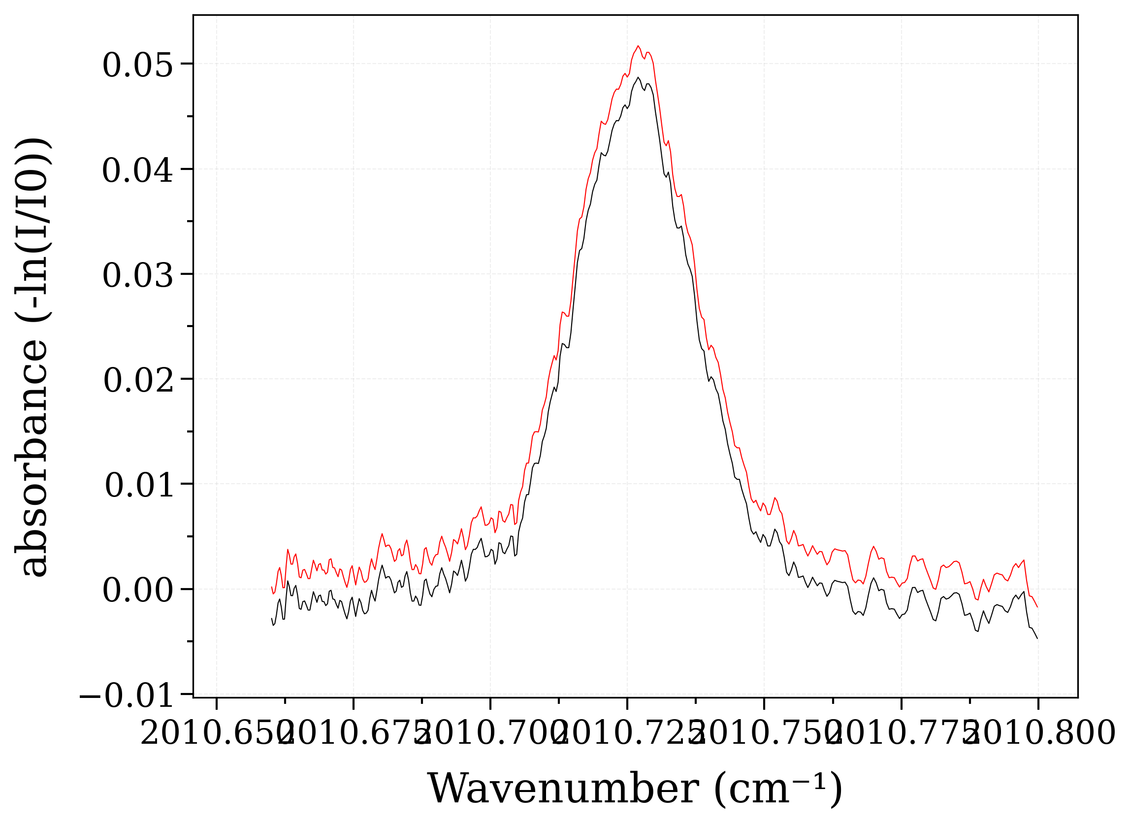
It seems the baseline is slightly offset (negative). Fix it with algebraic operations and show the difference

s.plot(nfig=2, show=False)
s += 0.003  # could have used an Astropy unit here too !
s.plot(nfig=2, color="r")

<matplotlib.lines.Line2D object at 0x7fbdf2a09480>

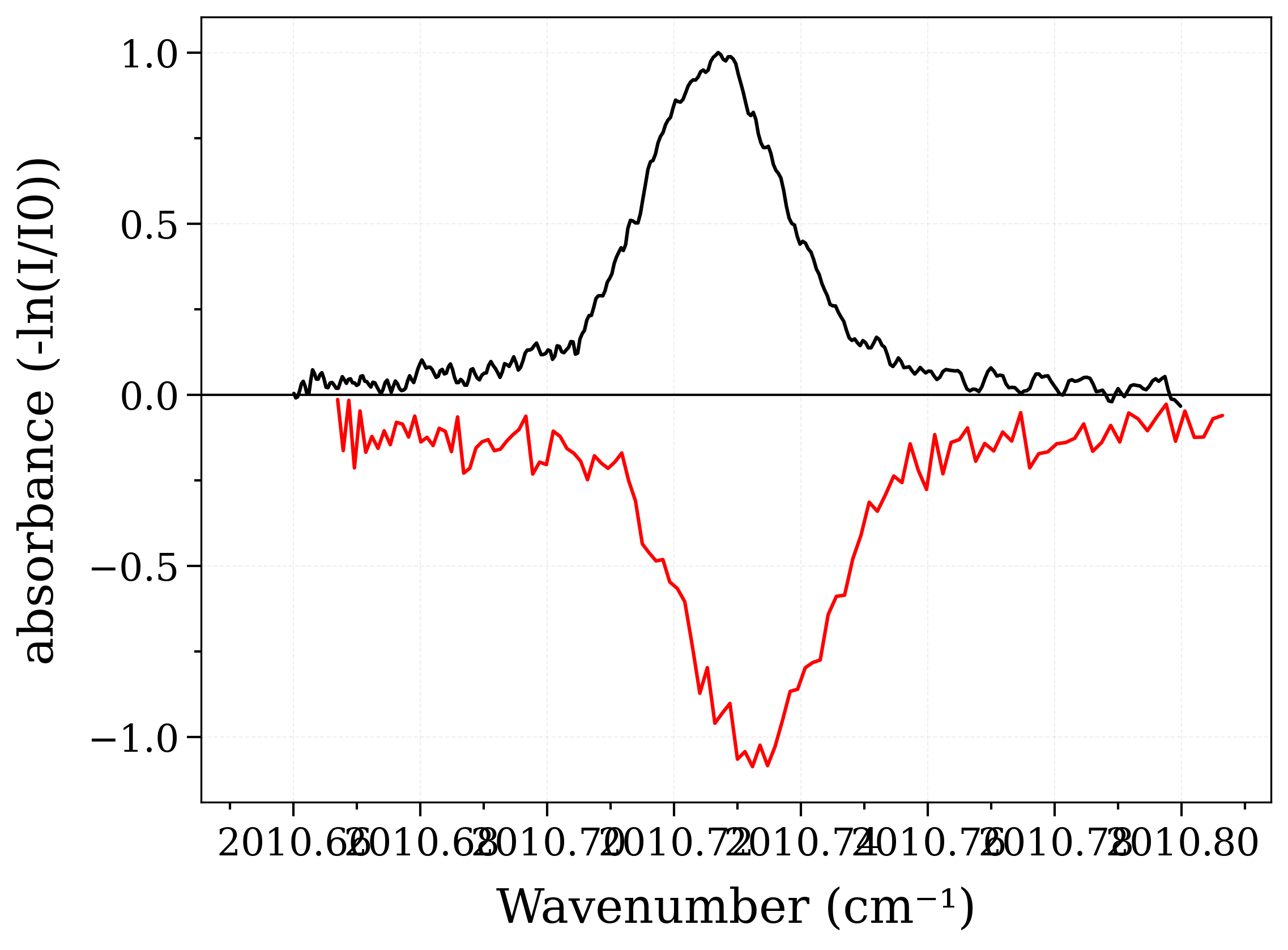
Some operations, such as crop, happen “in-place” by default, i.e. they modify the Spectrum. If you don’t want to modify the Spectrum make sure you specify inplace=False For instance we compare the current Spectrum to a mock-up new experimental spectrum obtained by adding some random noise (15%) on top of the the previous one, with some offset and a coarser grid.

Note the use of len(s) to get the number of spectral points

import matplotlib.pyplot as plt
import numpy as np

from radis.phys.units import Unit

s.normalize(inplace=False).plot(lw=1.5, show=False)
noise_array = 0.15 * (
    np.random.rand(len(s)) * Unit("")
)  # must be dimensioned to be multipled to spectra
noise_offset = np.random.rand(1) * 0.01
s2 = (-1 * (s.normalize(inplace=False) + noise_array)).offset(
    noise_offset, "cm-1", inplace=False
)
# Resample the spectrum on a coarser (1 every 3 points) grid
s2.resample(s2.get_wavenumber()[::3], inplace=True, energy_threshold=None)

plt.axhline(0)  # draw horizontal line
s2.plot(nfig="same", lw=1.5)

/home/docs/checkouts/readthedocs.org/user_builds/radis/checkouts/latest/radis/misc/warning.py:427: UnevenWaverangeWarning:

When resampling the spectrum, the new waverange had unequal spacing.


<matplotlib.lines.Line2D object at 0x7fbddb7efdc0>

Back to our original spectrum, we get the line positions using the max() or argmax() function

print("Maximum identified at ", s.argmax())

Maximum identified at  2010.7269449336343 1 / cm

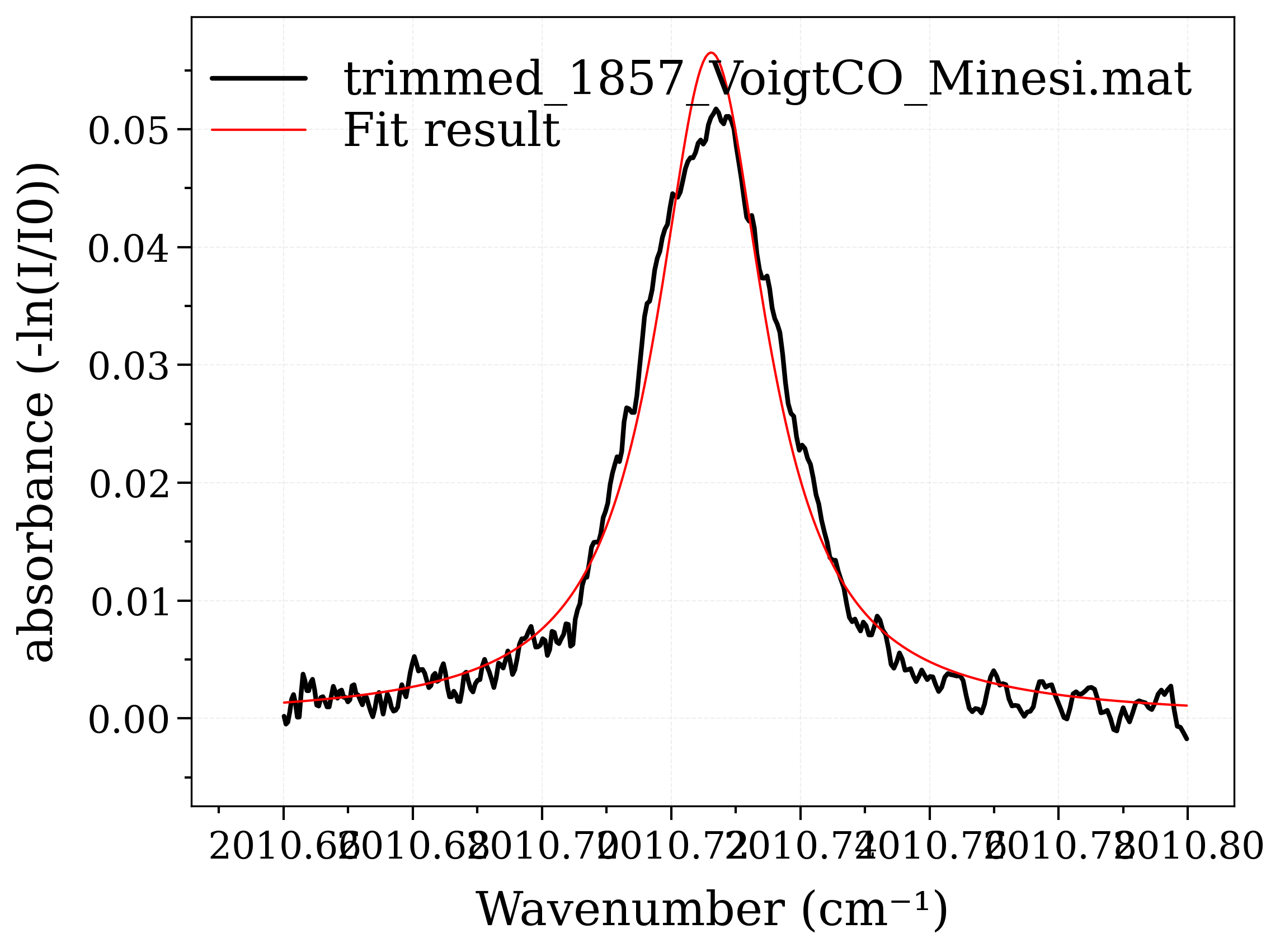
For a more accurate measurement of the line position, we fit a Lorentzian lineshape using Astropy & Specutil models (with straightforward Radis ==> Specutil conversion) and compare the fitted line center.

from astropy import units as u
from astropy.modeling import models
from specutils.fitting import fit_lines

# Fit the spectrum and calculate the fitted flux values (``y_fit``)
g_init = models.Lorentz1D(
    amplitude=s.max(), x_0=s.argmax(), fwhm=0.2
)  # see also models.Voigt1D
g_fit = fit_lines(s.to_specutils(), g_init)
w_fit = s.get_wavenumber() / u.cm
y_fit = g_fit(w_fit)

print("Fitted Line Center :  ", g_fit.x_0.value)

# Plot the original spectrum and the fitted.
import matplotlib.pyplot as plt

s.plot(lw=2, show=False)
plt.plot(w_fit, y_fit, label="Fit result")
plt.grid(True)
plt.legend()

Fitted Line Center :   2010.7261919753003

<matplotlib.legend.Legend object at 0x7fbde62a7970>

We can also mesure the area under the line :

import numpy as np

print("Absorbance of original line : ", s.get_integral("absorbance"))
print(
    "Absorbance of fitted line   :", np.trapz(y_fit, w_fit)
)  # negative because w_fit in descending order
#

Absorbance of original line :  0.001629699288083762
Absorbance of fitted line   : -0.0016606547425965664 1 / cm

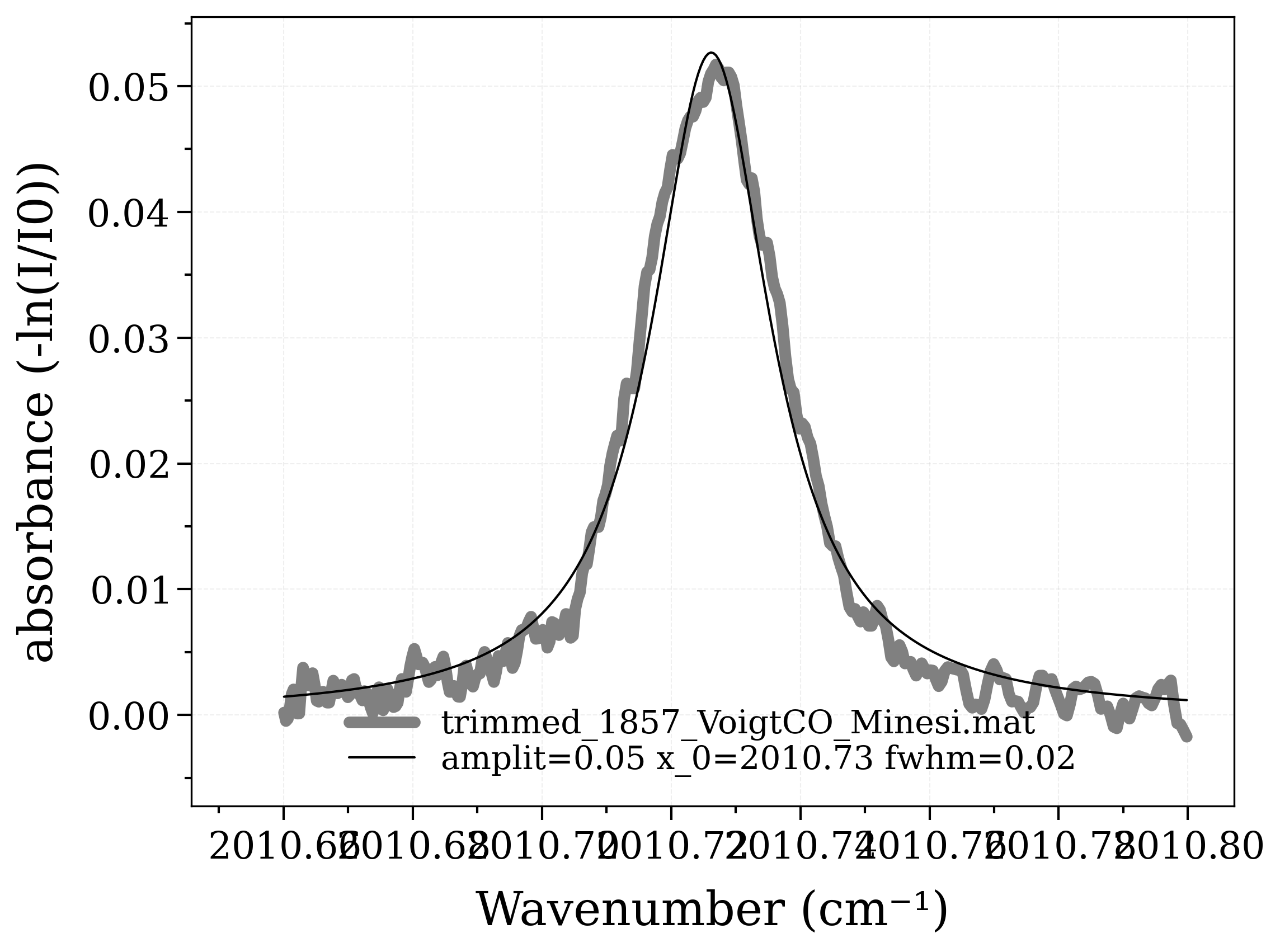
Finally note that the fitting routine can be achieved directly using the fit_model() function:

from astropy.modeling import models

s.fit_model(models.Lorentz1D(), plot=True)

([<Lorentz1D(amplitude=0.05267227 , x_0=2010.72621079 1 / cm, fwhm=0.02227926 1 / cm)>], [<Quantity 0.00060052>, <Quantity 0.00025259 1 / cm>, 0.00037279456823682285])

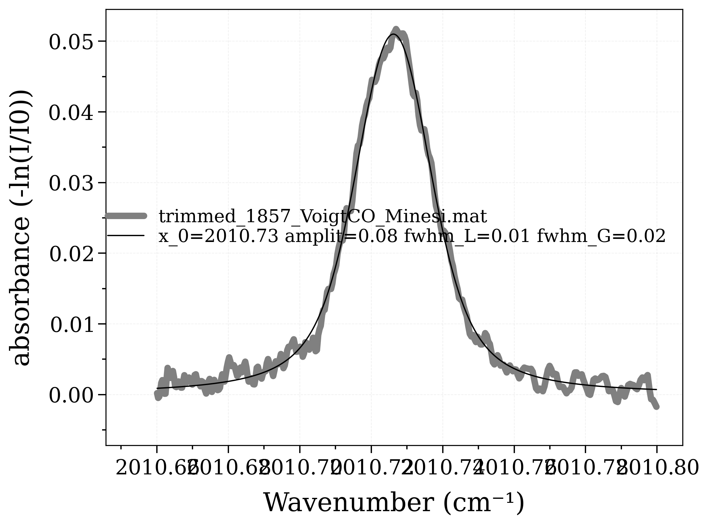
We see that fitting a Voigt profile yields substantially better results

from astropy.modeling import models

s.fit_model(models.Voigt1D(), plot=True)

([<Voigt1D(x_0=2010.72621028 1 / cm, amplitude_L=0.08047294 , fwhm_L=0.01364846 1 / cm, fwhm_G=0.01722931 1 / cm)>], [<Quantity 0.00011015 1 / cm>, <Quantity 0.0044678>, 0.000891958921859789, 0.0009052129810098868])