


RADIS-GPU Spectrum Calculation
RADIS provides GPU acceleration to massively speedup spectral computations. It uses the Vulkan API compute pipelines to perform parallel execution of spectral calculations
GPU calculations are handled by the gpuApp object, which takes care of initialization,
updating spectra, and freeing all GPU resources.
Generally GPU computations are memory bandwidth limited, meaning the computation time of
a single spectrum is determined by the time it takes to move the database data from host
(=CPU) to device (=GPU) memory. Because of this, GPU computations take place in two steps:
An initialization step, and one or many iteration step(s). The initialization step is performed during construction of the gpuApp object. During this step the database, as well as relevant initialization parameters,
are uploaded to the GPU. In the iteration step, iterate(), a new spectrum
with new parameters (T, p, etc) but relying on the same database is computed. This iteration can be repeated indefinitely
as long as the same database and spectral axis is used, resulting in extremely fast spectrum generation.
RADIS implements two functions that expose GPU functionality:
eq_spectrum_gpu()computes a single spectrum and returns. After generating the initial spectrum s, it can be updated many times using therecalc_gpu()method. Once the GPU is no longer needed, you have to free resources by calling theexit_gpu()method.eq_spectrum_gpu_interactive()computes a single spectrum and allows to interactively adjust parameters such as temperature, pressure, and composition, updating the spectrum in real time. Because the database only has to be transferred once, the updated spectra are calculated extremely fast.
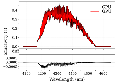
GPU computation is currently only supported for equilibrium spectra. It is likely that non-equilibrium spectra will be supported at some point in the future.
Single Spectrum
As mentioned above, the function eq_spectrum_gpu()
produces a single equilibrium spectrum using GPU acceleration. Consequent calls can then be to recalc_gpu(). Below is a usage example:
from radis import SpectrumFactory

sf = SpectrumFactory(
    2100,
    2400,  # cm-1
    molecule="CO2",
    isotope="1,2,3",
    wstep=0.002,
)

sf.fetch_databank("hitran") #for a fast demonstration
# sf.fetch_databank("hitemp", "2010") #for an accurate high-temperature demonstration
# sf.fetch_databank("hitemp") #latest hitemp version, slow download and parsing

T_list = [1000.0, 1500.0, 2000.0]

s = sf.eq_spectrum_gpu(
    Tgas=T_list[0],  # K
    pressure=1,  # bar
    mole_fraction=0.8,
    path_length=0.2,  # cm
)

s.apply_slit(0.5)#cm-1
s.plot("radiance", show=True)

for T in T_list[1:]:
    s.recalc_gpu(Tgas=T)
    show = (True if T == T_list[-1] else False)
    s.plot("radiance", show=show, nfig="same")

s.exit_gpu()
Examples using radis.lbl.SpectrumFactory.eq_spectrum_gpu
Interactive Spectrum
As mentioned before, computing the first GPU spectrum in a session takes a comparatively long time because the
entire database must be transferred to the GPU. The real power of GPU acceleration
becomes evident when computation times are not limited by data-transfer, i.e., when multiple
consecutive spectra are synthesized. One obvious use case would be the fitting of a spectrum.
Another one is interactive plotting, which can be done by calling
eq_spectrum_gpu_interactive(). A usage example is shown below:
from radis.tools.plot_tools import ParamRange
from radis import SpectrumFactory

sf = SpectrumFactory(
    2100,
    2400,  # cm-1
    molecule="CO2",
    isotope="1,2,3",
    wstep=0.002,
)

sf.fetch_databank("hitran")

s = sf.eq_spectrum_gpu_interactive(
    var="radiance",
    Tgas=ParamRange(300.0, 2500.0, 1100.0),  # K
    pressure=ParamRange(0.1, 2, 1),  # bar
    mole_fraction=ParamRange(0, 1, 0.8),
    path_length=ParamRange(0, 1, 0.2),  # cm
    slit_function=ParamRange(0, 1.5, 0.24),  # cm-1
    plotkwargs={"nfig": "same", "wunit": "nm"},
)
Note that eq_spectrum_gpu_interactive() replaces all of eq_spectrum_gpu(),
s.apply_slit(), and s.plot() seen in the earlier example, and for this reason the
syntax is a little bit different. For example, we directly pass the var keyword to
eq_spectrum_gpu_interactive() to specify which spectrum should be plotted, and keyword arguments to s.plot()
are passed through plotkwargs.
Quantities that are to be varied must be initialized by a
ParamRange() (valmin, valmax, valinit) object, which
takes the minimum value, maximum value, and init values of the scan range. Each ParamRange()
object will spawn a slider widget in the plot window with which the parameter can be
interactively adjusted. The algorithm is extremely fast for a large number of lines (>100M)
and will update with very low latency (<200ms typically). The code is not currently optimized
for large wavenumber ranges (>500cm-1) however, which may take a bit longer (up to a couple seconds),
provided the GPU didn’t run out of memory.
At this moment the application of the instrumental function is done on the CPU to benefit from all features
already implemented in apply_slit(). It is expected that these computations
will also move to the GPU at some point in the future.
Did you miss any feature implemented on GPU? Or support for your particular system? The GPU code is heavily under development, so drop us a visit on our GitHub and let us know what you’re looking for!