


Legacy vs recommended fitting examples
In this example, an experimental spectrum is fit using two fitting pipelines:
Legacy fitting module of
fit_spectrum(). You can find the gallery example featuring it at1 temperature fit.New fitting module of
fit_spectrum(), a new fitting interface for a more practical and interactive fitting experience. See1 temperature fit using new module
THe present code compare their overall performance, including number of loops, fitting time, and final residuals between experimental and best-fit spectra, as an indicator of fit accuracy.
Using database: HITRAN-CO2-TEST
'HITRAN-CO2-TEST':
{'info': 'HITRAN 2016 database, CO2, 1 main isotope (CO2-626), bandhead: 2380-2398 cm-1 (4165-4200 nm)', 'path': ['/home/docs/checkouts/readthedocs.org/user_builds/radis/checkouts/latest/radis/test/files/hitran_co2_626_bandhead_4165_4200nm.par'], 'format': 'hitran', 'levelsfmt': 'radis'}
Reference databank (2391.79-2399.14cm-1) has 0 lines in range (2391.69-2399.15cm-1) for isotope 2. Change your range or isotope options
/home/docs/checkouts/readthedocs.org/user_builds/radis/checkouts/latest/radis/misc/log.py:51: UserWarning: Reference databank (2391.79-2399.14cm-1) has 0 lines in range (2391.69-2399.15cm-1) for isotope 2. Change your range or isotope options
warn(msg)
0.03s - Loaded database
/home/docs/checkouts/readthedocs.org/user_builds/radis/checkouts/latest/radis/misc/warning.py:443: LinestrengthCutoffWarning: Estimated error after discarding lines is large: 0.07%. Consider reducing cutoff
warnings.warn(WarningType(message))
Calculating Equilibrium Spectrum
Physical Conditions
----------------------------------------
Tgas 300 K
isotope 1,2
medium air
mole_fraction 1
path_length 10 cm
pressure 0.001 bar
self_absorption True
species CO2
state X
wavenum_max 2399.1537 cm-1
wavenum_min 2391.6923 cm-1
Computation Parameters
----------------------------------------
Tref 296 K
add_at_used numpy
broadening_method voigt_poly
cutoff 1e-25 cm-1/(#.cm-2)
dbformat hitran
dbpath /home/docs/checkouts/readthedocs.org/user_builds/radis/checkouts/latest/radis/test/files/hitran_co2_...
diluent air
folding_thresh 1e-06
include_neighbouring_lines True
isatom False
isneutral None
lbfunc None
memory_mapping_engine auto
neighbour_lines 0 cm-1
optimization simple
parsum_mode full summation
pfsource default
potential_lowering None
pseudo_continuum_threshold 0
sparse_ldm True
truncation 1 cm-1
waveunit cm-1
wstep 0.001 cm-1
zero_padding 7463
----------------------------------------
0.02s - Spectrum calculated
/home/docs/checkouts/readthedocs.org/user_builds/radis/checkouts/latest/radis/misc/warning.py:443: LinestrengthCutoffWarning: Estimated error after discarding lines is large: 0.07%. Consider reducing cutoff
warnings.warn(WarningType(message))
/home/docs/checkouts/readthedocs.org/user_builds/radis/checkouts/latest/radis/misc/warning.py:443: LinestrengthCutoffWarning: Estimated error after discarding lines is large: 0.07%. Consider reducing cutoff
warnings.warn(WarningType(message))
Now starting the fitting process:
---------------------------------
/home/docs/checkouts/readthedocs.org/user_builds/radis/checkouts/latest/radis/tools/fitting.py:480: OptimizeWarning: Unknown solver options: disp
best = minimize(
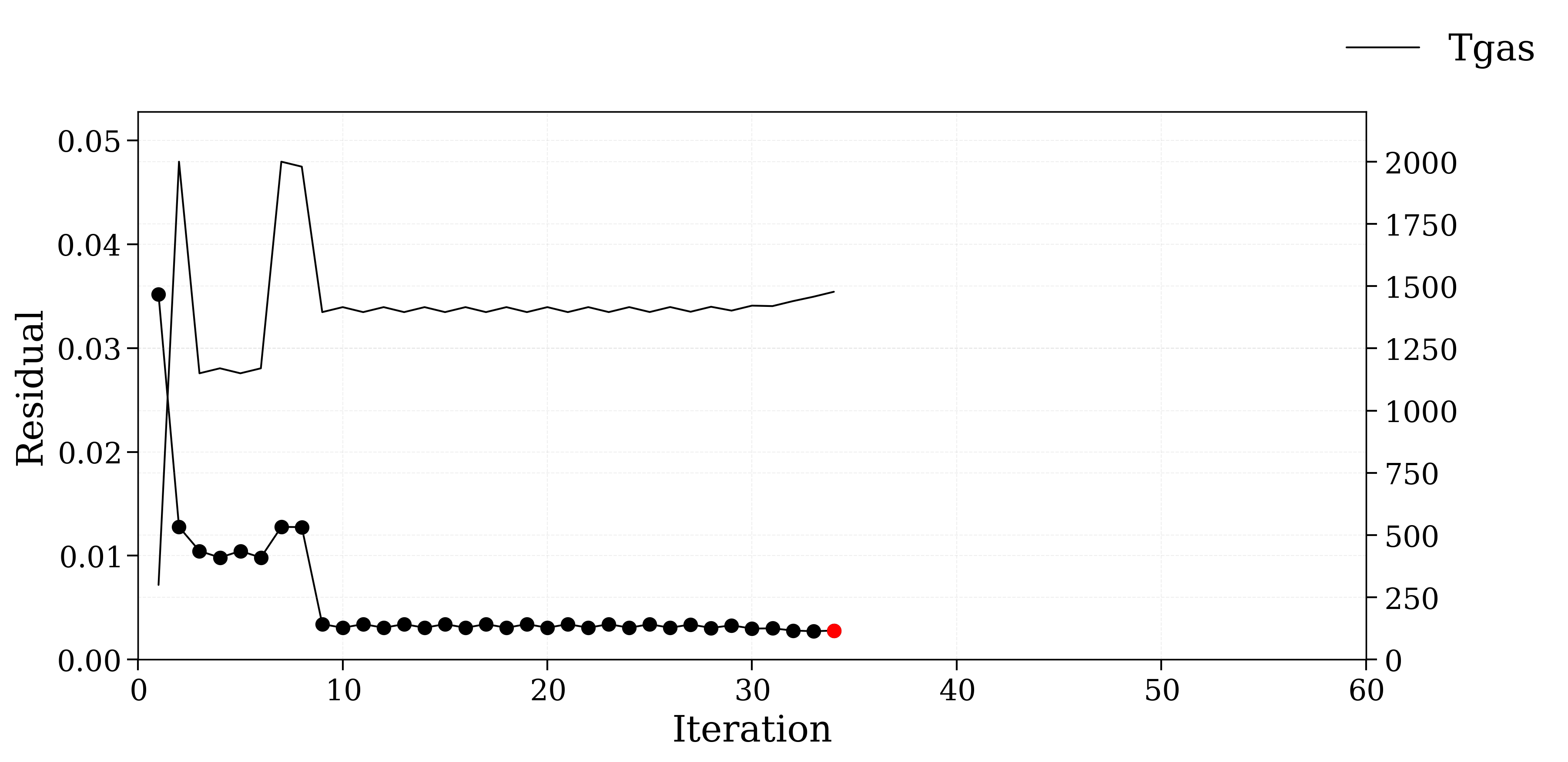
Tgas=1150.0, Residual: 0.0105 🏆
Tgas=1170.0, Residual: 0.0098 🏆
Tgas=1150.0, Residual: 0.0105
Tgas=1170.0, Residual: 0.0098 🏆
Tgas=2000.0, Residual: 0.0128
Tgas=1980.0, Residual: 0.0128
Tgas=1396.0, Residual: 0.0034 🏆
Tgas=1416.0, Residual: 0.0031 🏆
Tgas=1396.0, Residual: 0.0034
Tgas=1416.0, Residual: 0.0031 🏆
Tgas=1396.0, Residual: 0.0034
Tgas=1416.0, Residual: 0.0031 🏆
Tgas=1396.0, Residual: 0.0034
Tgas=1416.0, Residual: 0.0031 🏆
Tgas=1396.0, Residual: 0.0034
Tgas=1416.0, Residual: 0.0031 🏆
Tgas=1396.0, Residual: 0.0034
Tgas=1416.0, Residual: 0.0031 🏆
Tgas=1396.0, Residual: 0.0034
Tgas=1416.0, Residual: 0.0031 🏆
Tgas=1396.0, Residual: 0.0034
Tgas=1416.0, Residual: 0.0031 🏆
Tgas=1396.0, Residual: 0.0034
Tgas=1416.0, Residual: 0.0031 🏆
Tgas=1397.0, Residual: 0.0034
Tgas=1417.0, Residual: 0.0031 🏆
Tgas=1402.0, Residual: 0.0033
Tgas=1422.0, Residual: 0.0030 🏆
Tgas=1420.0, Residual: 0.0030
Tgas=1440.0, Residual: 0.0028 🏆
Tgas=1459.0, Residual: 0.0027 🏆
Tgas=1479.0, Residual: 0.0028
Init ['Tgas'] = [1150.]['']
Final ['Tgas'] = [1459.]['']
message: CONVERGENCE: NORM OF PROJECTED GRADIENT <= PGTOL
success: True
status: 0
fun: 0.0027304260508692786
x: [ 1.459e+03]
nit: 4
jac: [ 3.330e-06]
nfev: 32
njev: 16
hess_inv: <1x1 LbfgsInvHessProduct with dtype=float64>
Best ['Tgas'] = [1458.71148816][''] reached at iteration 32/32
0.03s - Loaded database
/home/docs/checkouts/readthedocs.org/user_builds/radis/checkouts/latest/radis/misc/curve.py:267: UserWarning: First spectrum has more resolution than 2nd. Reverse your spectra in interpolation/comparison for a better accuracy
warnings.warn(
/home/docs/checkouts/readthedocs.org/user_builds/radis/checkouts/latest/radis/misc/curve.py:267: UserWarning: First spectrum has more resolution than 2nd. Reverse your spectra in interpolation/comparison for a better accuracy
warnings.warn(
/home/docs/checkouts/readthedocs.org/user_builds/radis/checkouts/latest/radis/misc/curve.py:267: UserWarning: First spectrum has more resolution than 2nd. Reverse your spectra in interpolation/comparison for a better accuracy
warnings.warn(
/home/docs/checkouts/readthedocs.org/user_builds/radis/checkouts/latest/radis/misc/curve.py:267: UserWarning: First spectrum has more resolution than 2nd. Reverse your spectra in interpolation/comparison for a better accuracy
warnings.warn(
/home/docs/checkouts/readthedocs.org/user_builds/radis/checkouts/latest/radis/misc/curve.py:267: UserWarning: First spectrum has more resolution than 2nd. Reverse your spectra in interpolation/comparison for a better accuracy
warnings.warn(
/home/docs/checkouts/readthedocs.org/user_builds/radis/checkouts/latest/radis/misc/curve.py:267: UserWarning: First spectrum has more resolution than 2nd. Reverse your spectra in interpolation/comparison for a better accuracy
warnings.warn(
/home/docs/checkouts/readthedocs.org/user_builds/radis/checkouts/latest/radis/misc/curve.py:267: UserWarning: First spectrum has more resolution than 2nd. Reverse your spectra in interpolation/comparison for a better accuracy
warnings.warn(
/home/docs/checkouts/readthedocs.org/user_builds/radis/checkouts/latest/radis/misc/curve.py:267: UserWarning: First spectrum has more resolution than 2nd. Reverse your spectra in interpolation/comparison for a better accuracy
warnings.warn(
/home/docs/checkouts/readthedocs.org/user_builds/radis/checkouts/latest/radis/misc/curve.py:267: UserWarning: First spectrum has more resolution than 2nd. Reverse your spectra in interpolation/comparison for a better accuracy
warnings.warn(
/home/docs/checkouts/readthedocs.org/user_builds/radis/checkouts/latest/radis/misc/curve.py:267: UserWarning: First spectrum has more resolution than 2nd. Reverse your spectra in interpolation/comparison for a better accuracy
warnings.warn(
/home/docs/checkouts/readthedocs.org/user_builds/radis/checkouts/latest/radis/misc/curve.py:267: UserWarning: First spectrum has more resolution than 2nd. Reverse your spectra in interpolation/comparison for a better accuracy
warnings.warn(
/home/docs/checkouts/readthedocs.org/user_builds/radis/checkouts/latest/radis/misc/curve.py:267: UserWarning: First spectrum has more resolution than 2nd. Reverse your spectra in interpolation/comparison for a better accuracy
warnings.warn(
/home/docs/checkouts/readthedocs.org/user_builds/radis/checkouts/latest/radis/misc/curve.py:267: UserWarning: First spectrum has more resolution than 2nd. Reverse your spectra in interpolation/comparison for a better accuracy
warnings.warn(
/home/docs/checkouts/readthedocs.org/user_builds/radis/checkouts/latest/radis/misc/curve.py:267: UserWarning: First spectrum has more resolution than 2nd. Reverse your spectra in interpolation/comparison for a better accuracy
warnings.warn(
/home/docs/checkouts/readthedocs.org/user_builds/radis/checkouts/latest/radis/misc/curve.py:267: UserWarning: First spectrum has more resolution than 2nd. Reverse your spectra in interpolation/comparison for a better accuracy
warnings.warn(
/home/docs/checkouts/readthedocs.org/user_builds/radis/checkouts/latest/radis/misc/curve.py:267: UserWarning: First spectrum has more resolution than 2nd. Reverse your spectra in interpolation/comparison for a better accuracy
warnings.warn(
/home/docs/checkouts/readthedocs.org/user_builds/radis/checkouts/latest/radis/misc/curve.py:267: UserWarning: First spectrum has more resolution than 2nd. Reverse your spectra in interpolation/comparison for a better accuracy
warnings.warn(
[[Fit Statistics]]
# fitting method = L-BFGS-B
# function evals = 16
# data points = 1
# variables = 1
chi-square = 2.6824e-07
reduced chi-square = 2.6824e-07
Akaike info crit = -13.1313719
Bayesian info crit = -15.1313719
## Warning: uncertainties could not be estimated:
this fitting method does not natively calculate uncertainties
and numdifftools is not installed for lmfit to do this. Use
`pip install numdifftools` for lmfit to estimate uncertainties
with this fitting method.
[[Variables]]
Tgas: 1464.94931 (init = 1150)
/home/docs/checkouts/readthedocs.org/user_builds/radis/checkouts/latest/radis/misc/curve.py:240: UserWarning: Presence of NaN in curve_divide!
Think about interpolation=2
warnings.warn(
==================== PERFORMANCE COMPARISON BETWEEN 2 FITTING METHODS ====================
1. LAST RESIDUAL
- Old 1T fitting example: 0.0027304260508692786
- New fitting module: 0.000517921976887822
2. NUMBER OF FITTING LOOPS
- Old 1T fitting example: 32 loops
- New fitting module: 16 loops
3. TOTAL TIME TAKEN (s)
- Old 1T fitting example: 1.4849278926849365 s
- New fitting module: 2.6678354740142822 s
==========================================================================================
'\n\nFrom the comparative result above, which includes last residual, total time fitting and total number of\nfitting loops of each fitting method, we can see that under exactly the same ground-truth conditions,\nfitting method (L-BFGS-B) and fitting pipeline, we can see that the new fitting module provides a better\naccuracy, while requiring less fitting loops and time for execution.\n\nYou are free to change the experimental spectrum and its accompanied ground-truth conditions, but please\nmake sure to keep the same inputs between the two for a transparent comparative result.\n\n'
import time
import astropy.units as u
from radis import SpectrumFactory, load_spec, plot_diff
from radis.test.utils import getTestFile, setup_test_line_databases
from radis.tools.fitting import LTEModel
from radis.tools.new_fitting import fit_spectrum
# -------------------- OLD 1-TEMPERATURE FITTING EXAMPLE -------------------- #
setup_test_line_databases()
# fit range
wlmin = 4167
wlmax = 4180
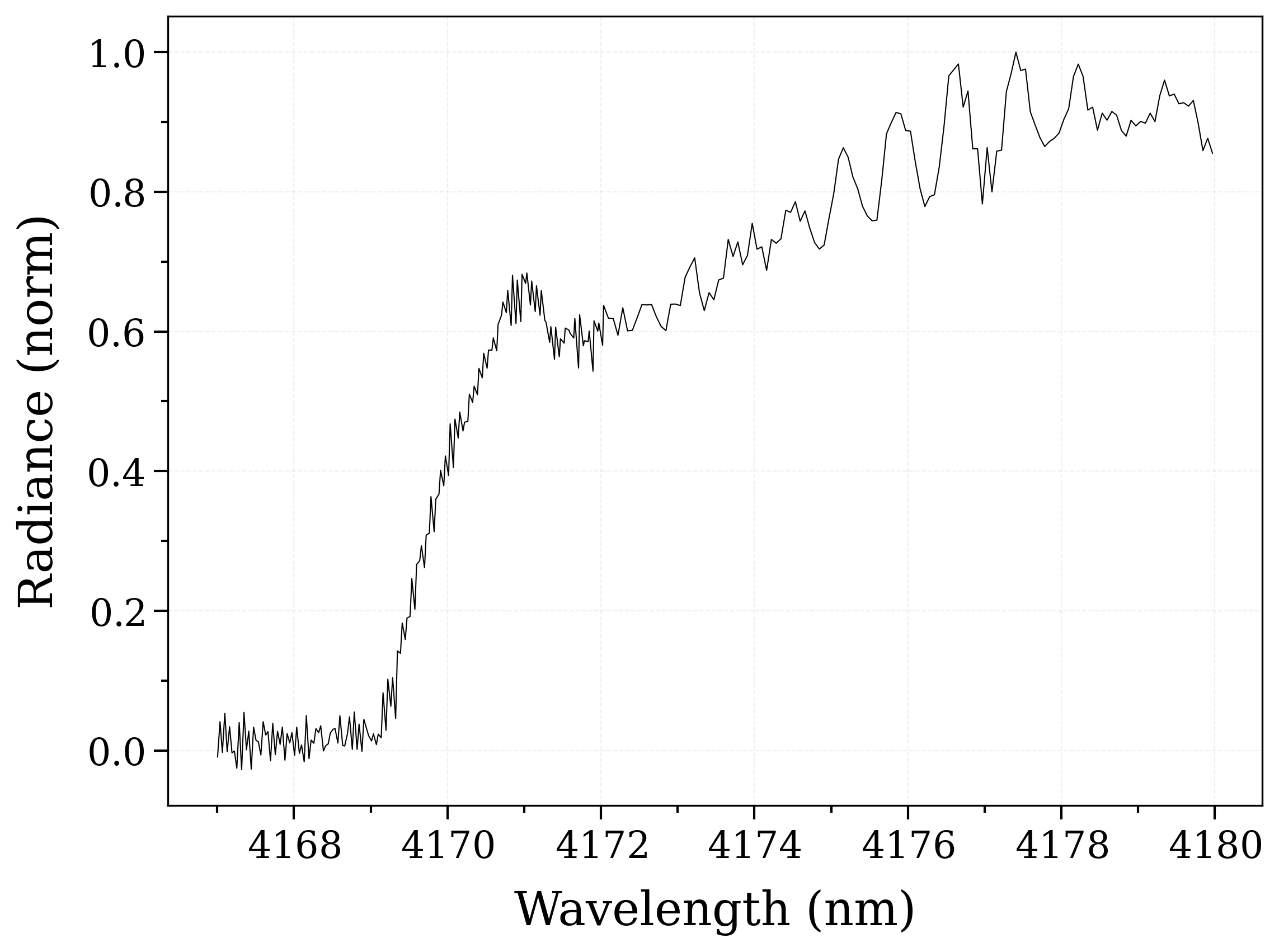
s_exp = (
load_spec(getTestFile("CO2_measured_spectrum_4-5um.spec"))
.crop(wlmin, wlmax, "nm")
.normalize()
.sort()
.offset(-0.2, "nm")
)
def LTEModel_withslitnorm(factory, fit_parameters, fixed_parameters):
s = LTEModel(factory, fit_parameters, fixed_parameters)
# we could also have added a fittable parameter, such as an offset,
# or made the slit width a fittable parameter.
# ... any parameter in model_input will be fitted.
# s.offset(model_input["offset"], 'nm')
s.apply_slit(1.4, "nm")
return s.take("radiance").normalize()
sf = SpectrumFactory(
wlmin * u.nm,
wlmax * u.nm,
wstep=0.001, # cm-1
pressure=1 * 1e-3, # bar
cutoff=1e-25,
isotope="1,2",
path_length=10, # cm-1
mole_fraction=1,
truncation=1, # cm-1
)
sf.warnings["MissingSelfBroadeningWarning"] = "ignore"
sf.warnings["HighTemperatureWarning"] = "ignore"
sf.load_databank("HITRAN-CO2-TEST")
begin_time_mark = time.time()
s_best, best = sf.fit_legacy(
s_exp.take("radiance"),
model=LTEModel_withslitnorm,
fit_parameters={
"Tgas": 300,
# "offset": 0
},
bounds={
"Tgas": [300, 2000],
# "offset": [-1, 1],
},
plot=True,
solver_options={
"maxiter": 15, # 👈 increase to let the fit converge
"ftol": 1e-15,
},
verbose=2,
)
end_time_mark = time.time()
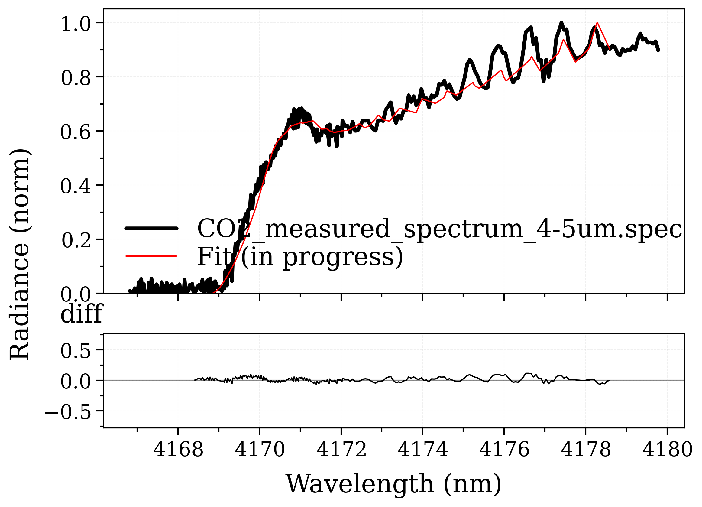
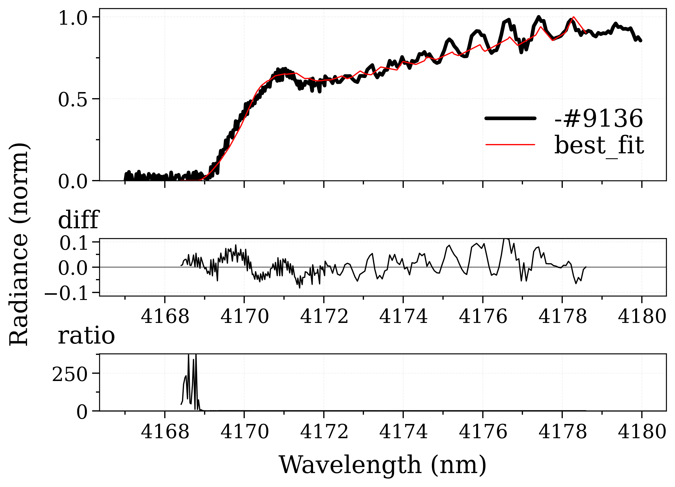
plot_diff(s_exp, s_best)
# Information to report later in comparison result
oldfitting_residual = best.fun
oldfitting_loops = best.nfev
oldfitting_time = end_time_mark - begin_time_mark
# ------------------------------------------------------------ #
# ---------------------------- NEW FITTING MODULE ---------------------------- #
# -------------------- Step 1. Load experimental spectrum -------------------- #
# Load an experimental spectrum. You can prepare yours, or fetch one of them in the radis/test/files directory.
my_spec = getTestFile("CO2_measured_spectrum_4-5um.spec")
s_experimental = load_spec(my_spec).offset(-0.2, "nm")
# -------------------- Step 2. Fill ground-truths and data -------------------- #
# Experimental conditions which will be used for spectrum modeling. Basically, these are known ground-truths.
experimental_conditions = {
"molecule": "CO2", # Molecule ID
"isotope": "1,2", # Isotope ID, can have multiple at once
"wmin": 4167
* u.nm, # Starting wavelength/wavenumber to be cropped out from the original experimental spectrum.
"wmax": 4180 * u.nm, # Ending wavelength/wavenumber for the cropping range.
"mole_fraction": 1, # Species mole fraction, from 0 to 1.
"pressure": 1
* 1e-3
* u.bar, # Total pressure of gas, in "bar" unit by default, but you can also use Astropy units.
"path_length": 10
* u.cm, # Experimental path length, in "cm" unit by default, but you can also use Astropy units.
"slit": "1.4 nm", # Experimental slit, must be a blank space separating slit amount and unit.
"wstep": 0.001, # Resolution of wavenumber grid, in cm-1.
"databank": "hitran", # Databank used for the spectrum calculation. Must be stated.
}
# List of parameters to be fitted, accompanied by their initial values.
fit_parameters = {
"Tgas": 1150, # Gas temperature, in K.
}
# List of bounding ranges applied for those fit parameters above.
# You can skip this step and let it use default bounding ranges, but this is not recommended.
# Bounding range must be at format [<lower bound>, <upper bound>].
bounding_ranges = {
"Tgas": [
300,
2000,
],
}
# Fitting pipeline setups.
fit_properties = {
"method": "lbfgsb", # Preferred fitting method. By default, "leastsq".
"fit_var": "radiance", # Spectral quantity to be extracted for fitting process, such as "radiance", "absorbance", etc.
"normalize": True, # Either applying normalization on both spectra or not.
"max_loop": 150, # Max number of loops allowed. By default, 200.
"tol": 1e-15, # Fitting tolerance, only applicable for "lbfgsb" method.
}
"""
For the fitting method, you can try one among 17 different fitting methods and algorithms of LMFIT,
introduced in `LMFIT method list <https://lmfit.github.io/lmfit-py/fitting.html#choosing-different-fitting-methods>`.
You can see the benchmark result of these algorithms here:
`RADIS Newfitting Algorithm Benchmark <https://github.com/radis/radis-benchmark/blob/master/manual_benchmarks/plot_newfitting_comparison_algorithm.py>`.
"""
# -------------------- Step 3. Run the fitting and retrieve results -------------------- #
# Conduct the fitting process!
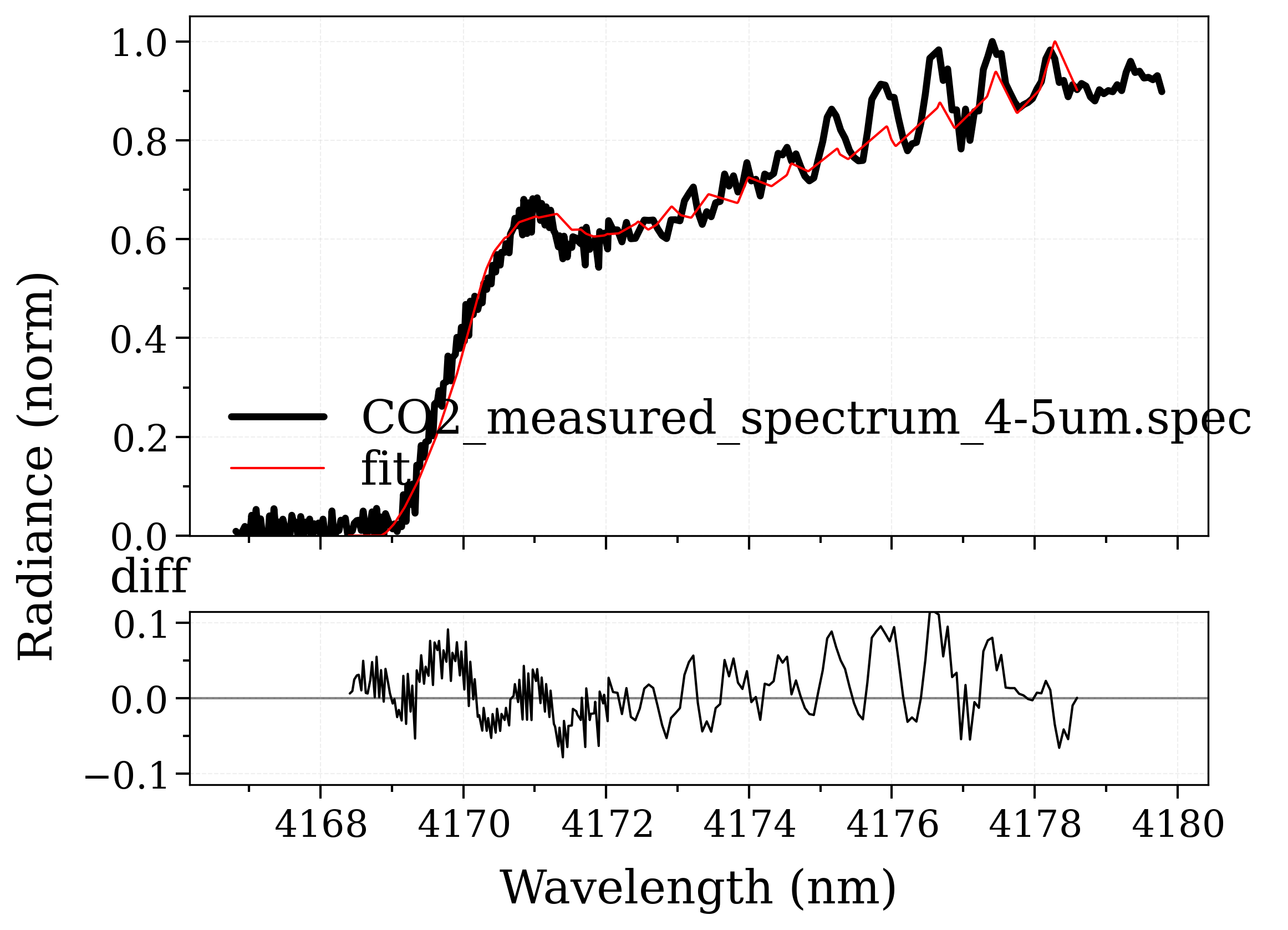
s_bestfit, result, log = fit_spectrum(
s_exp=s_experimental, # Experimental spectrum.
fit_params=fit_parameters, # Fit parameters.
bounds=bounding_ranges, # Bounding ranges for those fit parameters.
model=experimental_conditions, # Experimental ground-truths conditions.
pipeline=fit_properties, # Fitting pipeline references.
verbose=False, # If you want a clean result, stay False. If you want to see more about each loop, True.
)
# Information to report later in comparison result
newfitting_residual = log["residual"][-1]
newfitting_loops = result.nfev
newfitting_time = log["time_fitting"]
# ---------------------------------------------------------------------- #
# ---------------------------------- PERFORMANCE COMPARISON BETWEEN 2 FITTING METHODS ---------------------------------- #
print(
"\n\n\n==================== PERFORMANCE COMPARISON BETWEEN 2 FITTING METHODS ===================="
)
print("\n1. LAST RESIDUAL\n")
print(f"- Old 1T fitting example: \t{oldfitting_residual}")
print(f"- New fitting module: \t{newfitting_residual}")
print("\n2. NUMBER OF FITTING LOOPS\n")
print(f"- Old 1T fitting example: \t{oldfitting_loops} loops")
print(f"- New fitting module: \t{newfitting_loops} loops")
print("\n3. TOTAL TIME TAKEN (s)\n")
print(f"- Old 1T fitting example: \t{oldfitting_time} s")
print(f"- New fitting module: \t{newfitting_time} s")
print(
"\n==========================================================================================\n"
)
"""
From the comparative result above, which includes last residual, total time fitting and total number of
fitting loops of each fitting method, we can see that under exactly the same ground-truth conditions,
fitting method (L-BFGS-B) and fitting pipeline, we can see that the new fitting module provides a better
accuracy, while requiring less fitting loops and time for execution.
You are free to change the experimental spectrum and its accompanied ground-truth conditions, but please
make sure to keep the same inputs between the two for a transparent comparative result.
"""
Total running time of the script: (0 minutes 6.190 seconds)