


radis.spectrum.compare module
Summary
Functions to compare and plot comparison of Spectrum
objects
Routine Listings
- averageDistance(s1: Spectrum, s2: Spectrum, var='radiance')[source]
Return the average distance between two spectra. It’s important to note for fitting that if averageDistance(s1, s2)==0 then s1 = s2
- Parameters:
s1, s2 (Spectrum objects) – spectra to be compared
var (str, optional) – spectral quantity (ex: ‘radiance’, ‘transmittance’…)
- Returns:
distance – Average distance as in the following equation:
\[dist = \frac{\sqrt{\sum_i {(s1_i-s2_i)^2}}}{N}.\]- Return type:
float
- compare_spectra(first: Spectrum, other: Spectrum, spectra_only=False, plot=True, wunit='default', verbose=True, rtol=1e-05, ignore_nan=False, ignore_outliers=False, ignore_conditions=['calculation_time'], normalize=False, **kwargs) bool[source]
Compare Spectrum with another Spectrum object.
- Parameters:
first (type Spectrum) – a Spectrum to be compared
other (type Spectrum) – another Spectrum to compare with
spectra_only (boolean, or str) – if
True, only compares spectral quantities (in the same waveunit) and not lines or conditions. If str, compare a particular quantity name. If False, compare everything (including lines and conditions and populations). DefaultFalseplot (boolean) – if
True, use plot_diff to plot all quantities for the 2 spectra and the difference between them. DefaultTrue.wunit (‘nm’, ‘cm-1’, ‘default’) – in which wavespace to compare (and plot). If default, natural wavespace of first Spectrum is taken
rtol (float) – relative difference to use for spectral quantities comparison. absolute difference
atolis set to 0.ignore_nan (boolean) – if
True, nans are ignored when comparing spectral quantitiesignore_outliers (boolean, or float) –
if not False, outliers are discarded. i.e, output is determined by:
out = (~np.isclose(I, Ie, rtol=rtol, atol=0)).sum()/len(I) < ignore_outliers
ignore_conditions (list) – do not compare the metadata of these keys
normalize (bool) – Normalize the spectra to be plotted
- Other Parameters:
kwargs (dict) – arguments are forwarded to
plot_diff()- Returns:
equals – return True if spectra are equal (respective to tolerance defined by rtol and other input conditions)
- Return type:
boolean
Examples
Compare two Spectrum objects, or specifically the transmittance:
s1.compare_with(s2)
s1.compare_with(s2, 'transmittance')
Note that you can also simply use
s1 == s2, that usescompare_with()internally:s1 == s2 # will return True or False
- get_default_units(s1: Spectrum, s2: Spectrum, var=None, wunit='default', Iunit='default')[source]
Get
wunit, Iunit for var; compatible with both spectra s1 and s2- Parameters:
s1, s2 (Spectrum objects)
var (str, or None) – spectral quantity to plot (ex:
'abscoeff'). If None, plot the first one in the Spectrum from'radiance','radiance_noslit','transmittance', etc.wunit (
'default','nm','cm-1','nm_vac') – wavespace unit: wavelength air, wavenumber, wavelength vacuum. If'default', use first spectrum wunitIunit (str) – if
'default', use first spectrum unit
- Returns:
var (str) – variable (evaluated if input was
None)wunit, Iunit (str) – units (evaluated if input was
'default')
- get_diff(s1: Spectrum, s2: Spectrum, var, wunit='default', Iunit='default', resample=True, diff_window=0)[source]
Get the difference between 2 spectra.
Basically returns w1, I1 - I2 where (w1, I1) and (w2, I2) are the values of s1 and s2 for variable var. (w2, I2) is linearly interpolated if needed.
\[dI = I_1 - I_2\]- Parameters:
s1, s2 (Spectrum objects) – 2 spectra to compare.
var (str) – spectral quantity (ex:
'radiance','transmittance'…)wunit (
'nm','cm-1','nm_vac') – waveunit to compare in: wavelength air, wavenumber, wavelength vacuumIunit (str) – if
'default'use s1 unit for variable varmedium (‘air’, ‘vacuum’, default’) – propagating medium to compare in (if in wavelength)
- Other Parameters:
resample (bool) – if not
True, wavelength must be equals. Else, resamples2ons1if needed.diff_window (int) – If non 0, calculates diff by offsetting s1 by
diff_windownumber of units on either side, and returns the minimum. Compensates for experimental errors on the w axis. Default 0. (look up code for more details…)
- Returns:
w1, Idiff – difference interpolated on the wavespace range of the first Spectrum
- Return type:
array
Notes
Uses
curve_substract()internallySee also
get_ratio(),get_distance(),get_residual(),get_residual_integral(),plot_diff(),compare_with()
- get_distance(s1: Spectrum, s2: Spectrum, var, wunit='default', Iunit='default', resample=True, normalize=False, normalize_how='max')[source]
Get a regularized Euclidian distance between two spectra
s1ands2This regularized Euclidian distance minimizes the effect of a small shift in wavelength between the two spectra
\[D(w_1)[i] = \sqrt{ \sum_j (\hat{I_1}[i] - \hat{I_2}[j] )^2 + (\hat{w_1}[i] - \hat{w_2}[j])^2}\]Where values are normalized as:
\[\hat{A} = \frac{A}{max(A) - min(A)}\]If waveranges dont match,
s2is interpolated overs1.Warning
This is a distance on both the waverange and the intensity axis. It may be used to compensate for a small offset in your experimental spectrum (due to wavelength calibration, for instance) but can lead to wrong fits easily. Plus, it is very cost-intensive! Better use
get_residual()for an automatized procedure.- Parameters:
s1, s2 (Spectrum objects) –
Spectrumvar (str) – spectral quantity
wunit (
'nm','cm-1','nm_vac') – waveunit to compare in: wavelength air, wavenumber, wavelength vacuumIunit (str) – if
'default'use s1 unit for variable varmedium (‘air’, ‘vacuum’, default’) – propagating medium to compare in (if in wavelength)
- Other Parameters:
normalize (bool, or tuple) – if
True, normalize the two spectra before computing distance. If a tuple (ex:(4168, 4180)), normalize on this range only. The unit is that of the first Spectrum by default (usewunitto change). Ex:get_distance(s_exp, s_calc, var, normalize=(4178, 4180))
Default
Falsenormalize_how (
'max','area','mean') – how to normalize.'max'is the default but may not be suited for very noisy experimental spectra.'area'will normalize the integral to 1.'mean'will normalize by the mean amplitude value
Notes
Uses
curve_distance()internallySee also
get_diff(),get_ratio(),get_residual(),get_residual_integral(),plot_diff(),compare_with()
- get_ratio(s1: Spectrum, s2: Spectrum, var, wunit='default', Iunit='default', resample=True)[source]
Get the ratio between two spectra Basically returns w1, I1 / I2 where (w1, I1) and (w2, I2) are the values of s1 and s2 for variable var. (w2, I2) is linearly interpolated if needed.
\[R = I_1 / I_2\]- Parameters:
s1, s2 (Spectrum objects) –
Spectrumvar (str) – spectral quantity
wunit (
'nm','cm-1','nm_vac') – waveunit to compare in: wavelength air, wavenumber, wavelength vacuumIunit (str) – if
'default'use s1 unit for variable var
Notes
Uses
curve_divide()internallySee also
get_diff(),get_distance(),get_residual(),get_residual_integral(),plot_diff(),compare_with()
- get_residual(s1: Spectrum, s2: Spectrum, var, norm='L2', ignore_nan=False, diff_window=0, normalize=False, normalize_how='max', wunit='default', Iunit='default') float[source]
Returns L2 norm of
s1ands2For
I1,I2, the values of variablevarins1ands2, respectively, residual is calculated as:For
L2norm:\[res = \frac{\sqrt{\sum_i {(s_1[i]-s_2[i])^2}}}{N}.\]For
L1norm:\[res = \frac{\sqrt{\sum_i {|s_1[i]-s_2[i]|}}}{N}.\]- Parameters:
s1, s2 (
Spectrumobjects) – if not on the same range,s2is resampled ons1.var (str) – spectral array
norm (‘L2’, ‘L1’) – which norm to use
- Other Parameters:
ignore_nan (boolean) – if
True, ignorenanin the difference between s1 and s2 (ex: out of bound) when calculating residual. DefaultFalse. Note:get_residualwill still fail if there arenanin initial Spectrum.normalize (bool, or tuple) – if
True, normalize the two spectra before calculating the residual. If a tuple (ex:(4168, 4180)), normalize on this range only. The unit is that of the first Spectrum by default (usewunitto change). Ex:s_exp # in 'nm' s_calc # in 'cm-1' get_residual(s_exp, s_calc, normalize=(4178, 4180)) # interpreted as 'nm'
normalize_how (
'max','area','mean') – how to normalize.'max'is the default but may not be suited for very noisy experimental spectra.'area'will normalize the integral to 1.'mean'will normalize by the mean amplitude valuewunit (str) – used if normalized is a range. If
'default', use first spectrum unit.Iunit (str) – if
'default', use first spectrum unit
Notes
0 values for I1 yield nans except if I2 = I1 = 0
when s1 and s2 dont have the size wavespace range, they are automatically resampled through get_diff on ‘s1’ range
Implementation of
L2norm:np.sqrt((dI**2).sum())/len(dI)
Implementation of
L1norm:np.abs(dI).sum()/len(dI)
See also
get_diff(),get_ratio(),get_distance(),plot_diff(),get_residual_integral(),compare_with()
- get_residual_integral()[source]
Returns integral of the difference between two spectra s1 and s2, relatively to the integral of spectrum s1.
Compared to
get_residual(), this tends to cancel the effect of the gaussian noise of an experimental spectrum.res = trapezoid(I2-I1, w1) / trapezoid(I1, w1)
Note: when the considered variable is
transmittanceortransmittance_noslit, the upper integral is used (up to 1) to normalize the integral differenceres = trapezoid(I2-I1, w1) / trapezoid(1-I1, w1)
- Parameters:
s1, s2 (Spectrum objects) –
Spectrumvar (str) – spectral quantity
- Other Parameters:
ignore_nan (boolean) – if
True, ignore nan in the difference between s1 and s2 (ex: out of bound) when calculating residual. DefaultFalse. Note:get_residual_integralwill still fail if there are nan in initial Spectrum.wunit (str) – If
'default', use first spectrum unit.Iunit (str) – if
'default', use first spectrum unit
Notes
For I1, I2, the values of ‘var’ in s1 and s2, respectively, residual is calculated as:
res = trapezoid(I2-I1, w1) / trapezoid(I1, w1)
0 values for I1 yield nans except if I2 = I1 = 0
when s1 and s2 dont have the size wavespace range, they are automatically resampled through get_diff on ‘s1’ range
See also
get_diff(),get_ratio(),get_distance(),get_residual(),plot_diff(),compare_with()
- plot_diff(s1: Spectrum, s2: Spectrum, var=None, wunit='default', Iunit='default', resample=True, method='diff', diff_window=0, show_points=False, label1=None, label2=None, figsize=None, title=None, nfig=None, normalize=False, yscale='linear', verbose=True, save=False, show=True, show_residual=False, lw_multiplier=1, diff_scale_multiplier=1, discard_centile=0, plot_medium='vacuum_only', legendargs={'loc': 'best'}, show_ruler=False)[source]
Plot two spectra, and the difference between them.
method=allows you to plot the absolute difference, ratio, or both.If waveranges dont match,
s2is interpolated overs1.- Parameters:
s1, s2 (Spectrum objects)
var (str, or None) – spectral quantity to plot (ex:
'abscoeff'). If None, plot the first one in the Spectrum from'radiance','radiance_noslit','transmittance', etc.wunit (
'default','nm','cm-1','nm_vac') – wavespace unit: wavelength air, wavenumber, wavelength vacuum. If'default', use first spectrum wunitIunit (str) – if
'default', use first spectrum unitmethod (
'distance','diff','ratio', or list of them.) – If'diff', plot difference of the two spectra. If'distance', plot Euclidian distance (note that units are meaningless then) If'ratio', plot ratio of two spectra Default'diff'.Warning
with
'distance', calculation scales as ~N^2 with N the number of points in a spectrum (against ~N with'diff'). This can quickly override all memory.Can also be a list:
method=['diff', 'ratio']
normalize (bool) – Normalize the spectra to be plotted
- Other Parameters:
plot yscale
yscale: ‘linear’, ‘log diff_window: int
If non 0, calculates diff by offsetting s1 by
diff_windownumber of units on either side, and returns the minimum. Kinda compensates for experimental errors on the w axis. Default 0. (look up code to understand…)- show_points: boolean
if
True, make all points appear with ‘o’- label1, label2: str
curve names
- figsize
figure size
- nfig: int, str
figure number of name
- title: str
title
- verbose: boolean
if
True, plot stuff such as rescale ratio in normalize mode. DefaultTrue- save: str
Default is
False. By default won’t save anything, type the path of the destination if you want to save it (format in the name).- show: Bool
Default is
True. Will show the plots. You should switch toFalseif there are more than 20 calls of this function to avoid memory load during execution. IfFalse, you can show the plot(s) withplt.show()- show_residual: bool
if
True, calculates and shows on the graph the residual in L2 norm. Seeget_residual().diff_windowis used in the residual calculation too.normalizehas no effect.- diff_scale_multiplier: float
dilate the diff plot scale. Default
1- discard_centile: int
if not
0, discard the firsts and lasts centile when setting the limits of the diff window. Example:discard_centile=1 # --> discards the smallest 1% and largest 1% discard_centile=10 # --> discards the smallest 10% and largest 10%
Useful to remove spikes in a ratio, for instance. Note that this does not change the values of the residual. It’s just a plot feature. Default
0- plot_medium: bool,
'vacuum_only' if
Trueandwunitare wavelengths, plot the propagation medium in the xaxis label ([air]or[vacuum]). If'vacuum_only', plot only ifwunit=='nm_vac'. Default'vacuum_only'(prevents from inadvertently plotting spectra with different propagation medium on the same graph).- legendargs: dict
format arguments forwarded to the legend
- show_ruler: bool
if
True, add a ruler tool to the Matplotlib toolbar.Warning
still experimental in 0.9.30 ! Try it, feedback welcome !
- Returns:
fig (figure) – fig
[ax0, ax1] (axes) – spectra and difference axis
Examples
Simple use:
from radis import plot_diff
plot_diff(s10, s50)                # s10, s50 are two spectra
Advanced use, plotting the total power in the label, and getting the figure and axes handle to edit them afterwards:
Punit = 'mW/cm2/sr'
fig, axes = plot_diff(s10, s50, 'radiance_noslit', figsize=(18,6),
      label1='brd 10 cm-1, P={0:.2f} {1}'.format(s10.get_power(unit=Punit),Punit),
      label2='brd 50 cm-1, P={0:.2f} {1}'.format(s50.get_power(unit=Punit),Punit)
      )
# modify fig, axes..
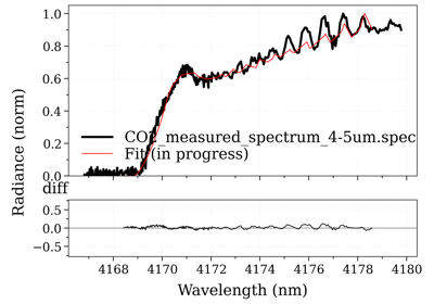
See an example in Compare two Spectra, which produces the output below:

If you wish to plot in a logscale, it can be done in the following way:
fig, [ax0, ax1] = plot_diff(s0, s1, normalize=False, verbose=False)
ylim0 = ax0.get_ybound()
ax0.set_yscale("log")
ax0.set_ybound(ylim0)
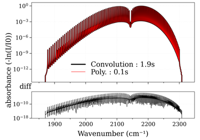
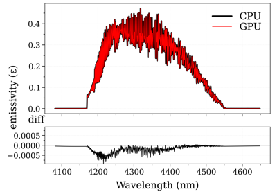
Performance increase of broadening_methods and LDM optimizations.
Performance increase of broadening_methods and LDM optimizations.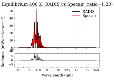
Compare OH(A-X) electronic spectra: RADIS vs Specair
Compare OH(A-X) electronic spectra: RADIS vs Specair
Calculate and Compare Spectra for Multiple Molecules
Calculate and Compare Spectra for Multiple MoleculesSee also
get_diff(),get_ratio(),get_distance(),get_residual(),compare_with()