Use different plot themes

Shows how to customize plot styles, using seaborn , matplotlib or publib

Examples

To change it in your user script, set the keys of the "plot" bloc in radis.config :

import radis
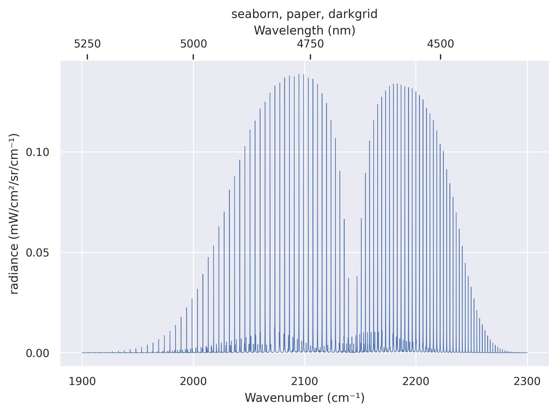
radis.config["plot"]["plotlib"] = "seaborn"
radis.config["plot"]["context"] = "paper"
radis.config["plot"]["style"] = "darkgrid"

To change your default settings, edit the ~/radis.json Configuration file

See Also

set_style(), fix_style(),

import matplotlib.pyplot as plt

import radis

plt.close("all")
s = radis.spectrum_test()

for plotlib, context, style in [
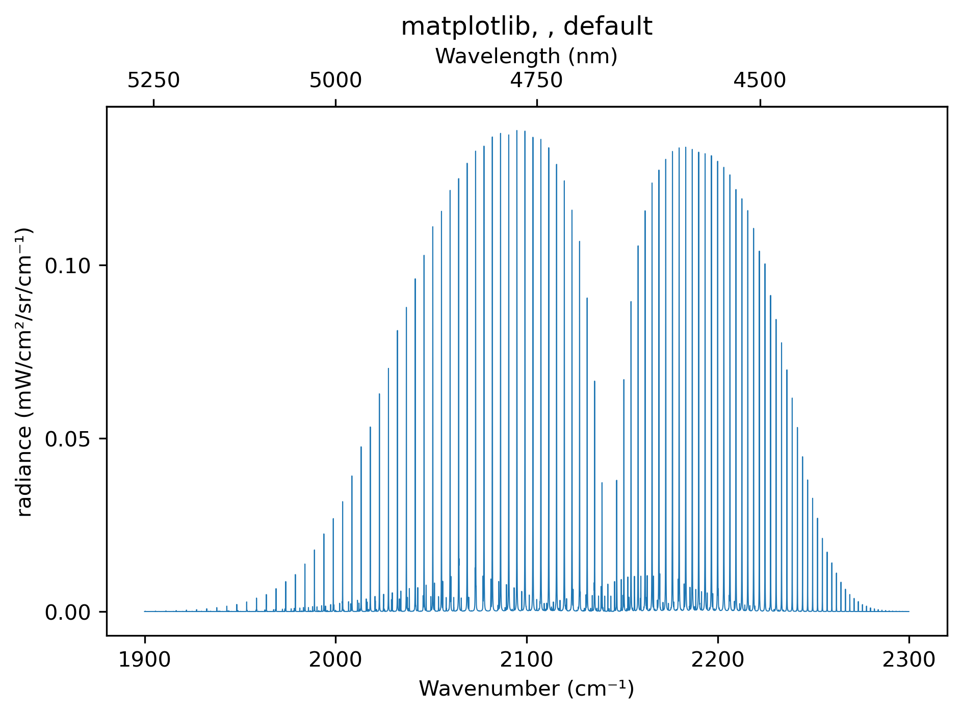
    ("matplotlib", "", "default"),
    ("seaborn", "paper", "darkgrid"),
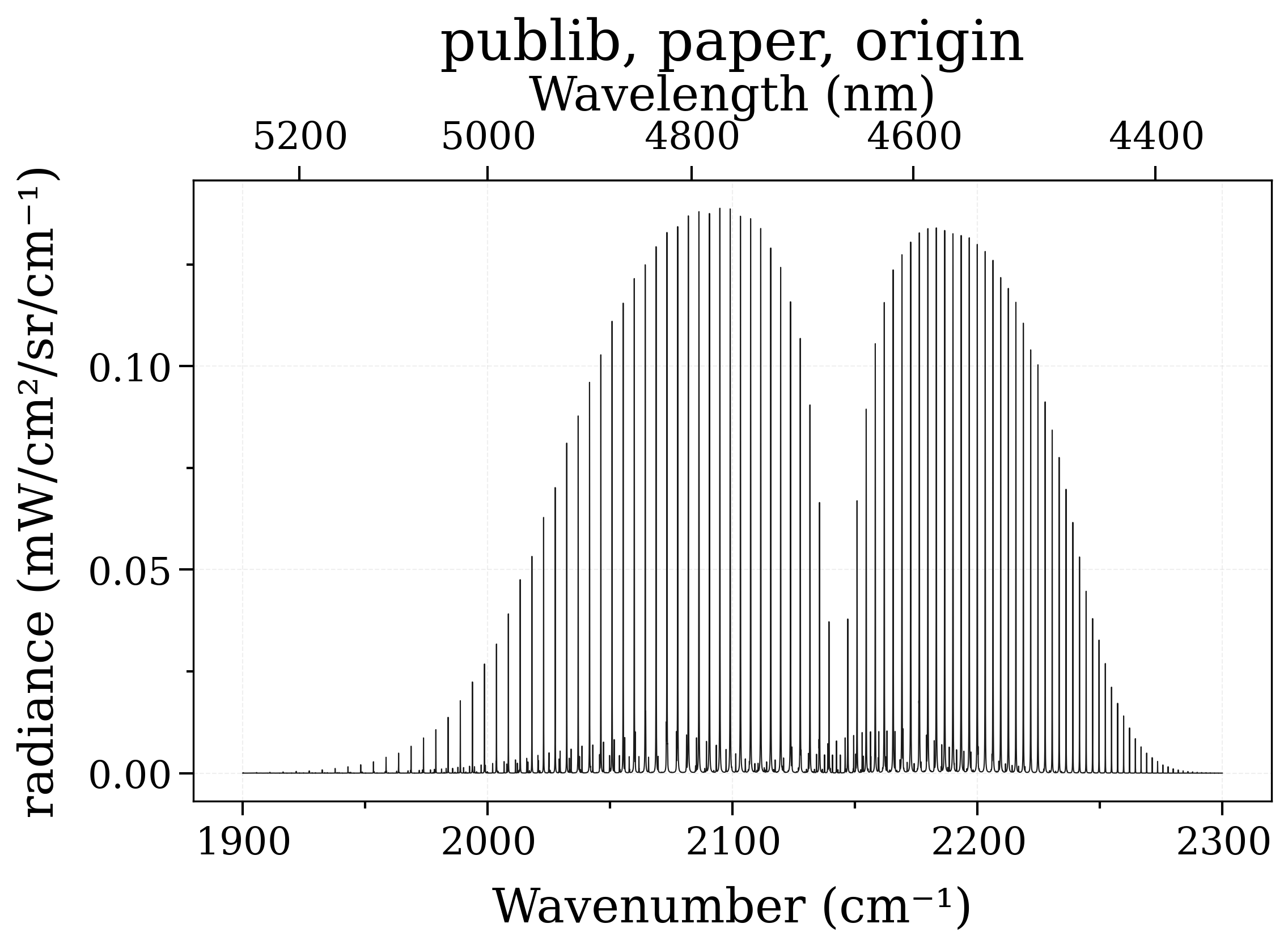
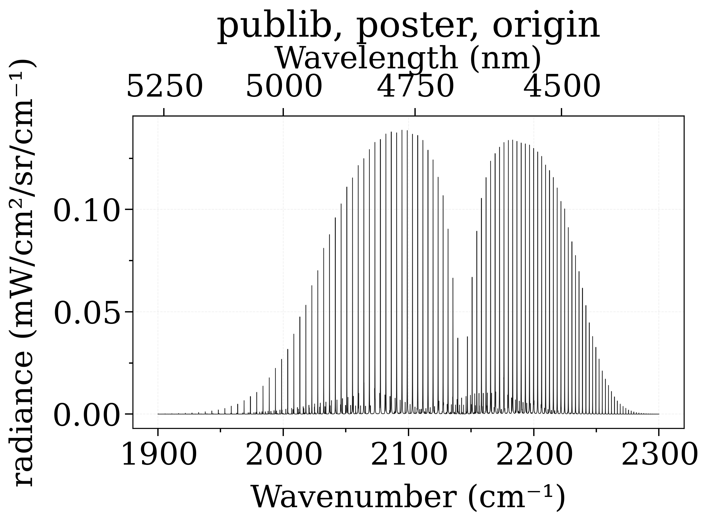
    ("publib", "paper", "origin"),
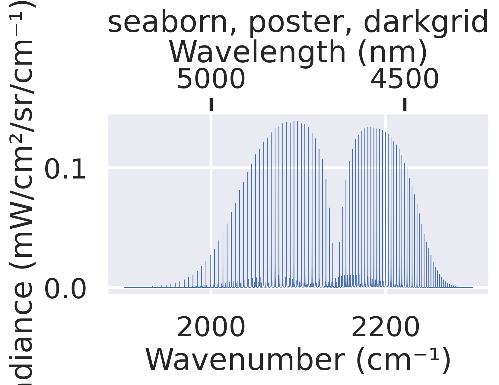
    ("seaborn", "poster", "darkgrid"),
    ("publib", "poster", "origin"),
]:
    radis.config["plot"]["plotlib"] = plotlib
    radis.config["plot"]["context"] = context
    radis.config["plot"]["style"] = style
    s.plot()
    plt.title(", ".join(f"{v}" for v in radis.config["plot"].values()))
    plt.tight_layout()

• 
• 
• 
• 
• 

--------------------------------------------------------------------------------
CO - HITRAN - Downloading database
--------------------------------------------------------------------------------

Download:
- All files already downloaded.

Caching to HDF5/H5 format:
- All files already cached.
0.03s - Loaded database
Calculating Equilibrium Spectrum
Physical Conditions
----------------------------------------
   Tgas                 700 K
   isotope              1,2,3
   medium               air
   mole_fraction        0.1
   path_length          1 cm
   pressure             1.01325 bar
   self_absorption      True
   species              CO
   state                X
   wavenum_max          2300.0000 cm-1
   wavenum_min          1900.0000 cm-1
Computation Parameters
----------------------------------------
   Tref                 296 K
   add_at_used          numpy
   broadening_method    voigt_poly
   cutoff               1e-27 cm-1/(#.cm-2)
   dbformat             hitran
   dbpath               /home/docs/.radisdb/hitran/CO.hdf5
   diluent              air
   folding_thresh       1e-06
   include_neighbouring_lines  True
   isatom               False
   isneutral            None
   lbfunc               None
   memory_mapping_engine  auto
   neighbour_lines      0 cm-1
   optimization         simple
   parsum_mode          full summation
   pfsource             default
   potential_lowering   None
   pseudo_continuum_threshold  0
   sparse_ldm           True
   truncation           50 cm-1
   waveunit             cm-1
   wstep                0.01 cm-1
   zero_padding         40002
----------------------------------------
0.05s - Spectrum calculated

You can also choose to not show the figure immediately, and instead return the Matplotlib or Plotly object. This allows for advanced customization (e.g., modifying the matplotlib figure).

fig, ax = s.plot("radiance_noslit", plotting_library="matplotlib", show=False)

ax.set_xlabel("Updated X-axis Label")
ax.set_ylabel("Updated Y-axis Label")
ax.grid(True, linestyle=":", linewidth=1)
ax.set_facecolor("beige")

fig.gcf().set_size_inches(8.6, 5)  # Resize
fig.gcf().set_dpi(150)  # Change DPI
# Then Show
fig.show()