


Performance increase of broadening_methods and LDM optimizations.
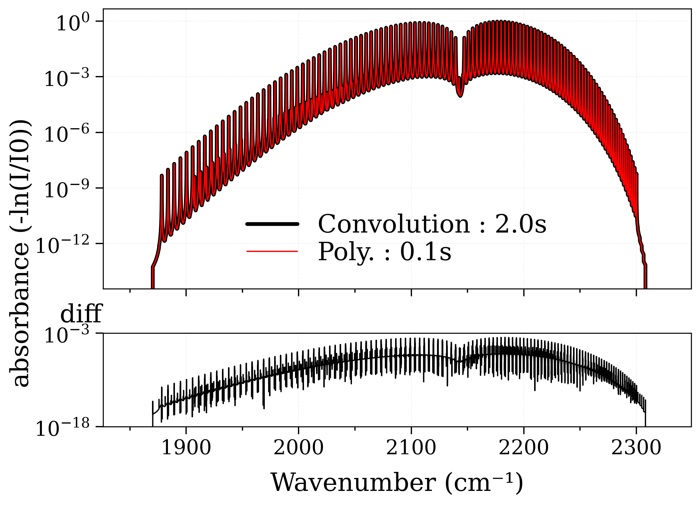
Auto-download, calculate, and compare CO spectra calculated with several numerical approximation of the Voigt functions. We also show that the LDM optimization (“simple” or “min-RMS”) leads to a significantly faster computation for almost no impact on the Voigt computation.
from radis import SpectrumFactory, plot_diff
trunc_ref = 8
conditions = {
"molecule": "CO",
"wavenum_min": 1850,
"wavenum_max": 2325,
# "molecule": "H2O", #un-comment these lines to try with H2O
# "wavelength_min": 2400,
# "wavelength_max": 3000,
"path_length": 0.1,
"mole_fraction": 0.2,
"isotope": 1, # or "1,2" or "all"
"pressure": 1,
"wstep": 0.002,
# also measure interpolation time
"truncation": trunc_ref, # cm-1; Default value is 50 cm-1 but the value is decreased here to accelerate the execution of this example
"cutoff": 1e-27, # cm-1/(#.cm-2); Default is 1e-27
}
Tgas = 400
databank, database = "hitran", "default"
# databank, database = = "hitemp", "2010" #for H2O, on your machine (will take longer to compute the reference spectrum)
############## Reference spectrum - No optimization used ##############
conditions["optimization"] = None
## Using a convolution of Gaussian and Lorentzian, no optimization
conditions["broadening_method"] = (
"convolve" # Voigt = numpy.convolve("Gaussian", "Lorentzian")
)
sf = SpectrumFactory(**conditions)
sf.fetch_databank(databank)
s_conv = sf.eq_spectrum(Tgas=Tgas)
s_conv.name = f"Convolution : {s_conv.c['calculation_time']:.1f}s"
# Using a polynomial approximation, no optimization
conditions["broadening_method"] = (
"voigt_poly" # Voigt = polynomial approximation derived from Whithing
)
sf = SpectrumFactory(**conditions)
sf.fetch_databank(databank, database=database)
s_poly = sf.eq_spectrum(Tgas=Tgas)
s_poly.name = f"Poly. : {s_poly.c['calculation_time']:.1f}s"
# Compare the spectra
plot_diff(
s_conv,
s_poly,
var="absorbance",
yscale="log",
# yscale="linear",
)
############## Using LDM optimization ##############
"""
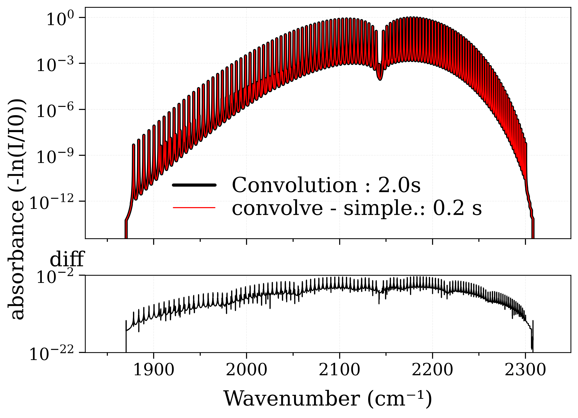
The objective of this section is to show how fast are the LDM optimizations.
The calculated spectra are compared to a reference (no optimization) where the
Voigts are calculated via numpy.convolve of a Gaussian and a Lorentzian.
**Conclusions:**
Using the 'linear' LDM optimization, it takes significantly less time to compute
the spectrum, whatever the broadening method employed. The relative difference is
always smaller than diff/ref < 1e-6. This difference can be improved by
changing from 'LDM = linear' to 'LDM = min-RMS' for a small cost in time.
"""
s_ref = s_conv
LDM_dic = {}
for method in ["convolve", "voigt_poly", "fft"]:
for LDM in ["simple", "min-RMS"]:
conditions["optimization"] = LDM
conditions["broadening_method"] = method
if method == "fft":
conditions["truncation"] = None
else:
conditions["truncation"] = s_ref.conditions[
"truncation"
] # cm-1 (Default value = 50)
sf = SpectrumFactory(**conditions)
sf.fetch_databank(databank)
s = sf.eq_spectrum(Tgas=Tgas)
s.name = f"{method} - {LDM}.: {s.c['calculation_time']:.1f} s"
LDM_dic[f"{LDM}_{method}"] = s
# Compare the spectrum to the reference
plot_diff(s_ref, s, "absorbance", yscale="log")


--------------------------------------------------------------------------------
CO - HITRAN - Downloading database
--------------------------------------------------------------------------------

Download:
- Downloading all isotopes for CO

Downloading isotopes:   0%|          | 0/9 [00:00<?, ?it/s]
Downloading isotopes:  11%|█         | 1/9 [00:00<00:02,  2.92it/s]
Downloading isotopes:  22%|██▏       | 2/9 [00:00<00:02,  3.15it/s]
Downloading isotopes:  33%|███▎      | 3/9 [00:00<00:01,  3.25it/s]
Downloading isotopes:  44%|████▍     | 4/9 [00:01<00:01,  3.28it/s]
Downloading isotopes:  56%|█████▌    | 5/9 [00:01<00:01,  3.29it/s]
Downloading isotopes:  67%|██████▋   | 6/9 [00:01<00:00,  3.47it/s]
Downloading isotopes: 100%|██████████| 9/9 [00:01<00:00,  5.01it/s]

HITRAN database download complete
Added HITRAN-CO database in /home/docs/radis.json
2.00s - Loaded database
Calculating Equilibrium Spectrum
Physical Conditions
----------------------------------------
   Tgas                 400 K
   isotope              1
   medium               air
   mole_fraction        0.2
   path_length          0.1 cm
   pressure             1 bar
   self_absorption      True
   species              CO
   state                X
   wavenum_max          2325.0000 cm-1
   wavenum_min          1850.0000 cm-1
Computation Parameters
----------------------------------------
   Tref                 296 K
   add_at_used
   broadening_method    convolve
   cutoff               1e-27 cm-1/(#.cm-2)
   dbformat             hitran
   dbpath
   diluent              air
   folding_thresh       1e-06
   include_neighbouring_lines  True
   isatom               False
   isneutral            None
   lbfunc               None
   memory_mapping_engine  auto
   neighbour_lines      0 cm-1
   optimization         None
   parsum_mode          full summation
   pfsource             default
   potential_lowering   None
   pseudo_continuum_threshold  0
   sparse_ldm           True
   truncation           8 cm-1
   waveunit             cm-1
   wstep                0.002 cm-1
   zero_padding         237501
----------------------------------------
2.00s - Spectrum calculated
--------------------------------------------------------------------------------
CO - HITRAN - Downloading database
--------------------------------------------------------------------------------

Download:
- All files already downloaded.

Caching to HDF5/H5 format:
- All files already cached.
0.03s - Loaded database
Calculating Equilibrium Spectrum
Physical Conditions
----------------------------------------
   Tgas                 400 K
   isotope              1
   medium               air
   mole_fraction        0.2
   path_length          0.1 cm
   pressure             1 bar
   self_absorption      True
   species              CO
   state                X
   wavenum_max          2325.0000 cm-1
   wavenum_min          1850.0000 cm-1
Computation Parameters
----------------------------------------
   Tref                 296 K
   add_at_used
   broadening_method    voigt_poly
   cutoff               1e-27 cm-1/(#.cm-2)
   dbformat             hitran
   dbpath               /home/docs/.radisdb/hitran/CO.h5
   diluent              air
   folding_thresh       1e-06
   include_neighbouring_lines  True
   isatom               False
   isneutral            None
   lbfunc               None
   memory_mapping_engine  auto
   neighbour_lines      0 cm-1
   optimization         None
   parsum_mode          full summation
   pfsource             default
   potential_lowering   None
   pseudo_continuum_threshold  0
   sparse_ldm           True
   truncation           8 cm-1
   waveunit             cm-1
   wstep                0.002 cm-1
   zero_padding         237501
----------------------------------------
0.17s - Spectrum calculated
--------------------------------------------------------------------------------
CO - HITRAN - Downloading database
--------------------------------------------------------------------------------

Download:
- All files already downloaded.

Caching to HDF5/H5 format:
- All files already cached.
0.03s - Loaded database
Calculating Equilibrium Spectrum
Physical Conditions
----------------------------------------
   Tgas                 400 K
   isotope              1
   medium               air
   mole_fraction        0.2
   path_length          0.1 cm
   pressure             1 bar
   self_absorption      True
   species              CO
   state                X
   wavenum_max          2325.0000 cm-1
   wavenum_min          1850.0000 cm-1
Computation Parameters
----------------------------------------
   Tref                 296 K
   add_at_used          numpy
   broadening_method    convolve
   cutoff               1e-27 cm-1/(#.cm-2)
   dbformat             hitran
   dbpath               /home/docs/.radisdb/hitran/CO.h5
   diluent              air
   folding_thresh       1e-06
   include_neighbouring_lines  True
   isatom               False
   isneutral            None
   lbfunc               None
   memory_mapping_engine  auto
   neighbour_lines      0 cm-1
   optimization         simple
   parsum_mode          full summation
   pfsource             default
   potential_lowering   None
   pseudo_continuum_threshold  0
   sparse_ldm           True
   truncation           8 cm-1
   waveunit             cm-1
   wstep                0.002 cm-1
   zero_padding         237501
----------------------------------------
0.22s - Spectrum calculated
--------------------------------------------------------------------------------
CO - HITRAN - Downloading database
--------------------------------------------------------------------------------

Download:
- All files already downloaded.

Caching to HDF5/H5 format:
- All files already cached.
0.03s - Loaded database
Calculating Equilibrium Spectrum
Physical Conditions
----------------------------------------
   Tgas                 400 K
   isotope              1
   medium               air
   mole_fraction        0.2
   path_length          0.1 cm
   pressure             1 bar
   self_absorption      True
   species              CO
   state                X
   wavenum_max          2325.0000 cm-1
   wavenum_min          1850.0000 cm-1
Computation Parameters
----------------------------------------
   Tref                 296 K
   add_at_used          numpy
   broadening_method    convolve
   cutoff               1e-27 cm-1/(#.cm-2)
   dbformat             hitran
   dbpath               /home/docs/.radisdb/hitran/CO.h5
   diluent              air
   folding_thresh       1e-06
   include_neighbouring_lines  True
   isatom               False
   isneutral            None
   lbfunc               None
   memory_mapping_engine  auto
   neighbour_lines      0 cm-1
   optimization         min-RMS
   parsum_mode          full summation
   pfsource             default
   potential_lowering   None
   pseudo_continuum_threshold  0
   sparse_ldm           True
   truncation           8 cm-1
   waveunit             cm-1
   wstep                0.002 cm-1
   zero_padding         237501
----------------------------------------
0.22s - Spectrum calculated
--------------------------------------------------------------------------------
CO - HITRAN - Downloading database
--------------------------------------------------------------------------------

Download:
- All files already downloaded.

Caching to HDF5/H5 format:
- All files already cached.
0.03s - Loaded database
Calculating Equilibrium Spectrum
Physical Conditions
----------------------------------------
   Tgas                 400 K
   isotope              1
   medium               air
   mole_fraction        0.2
   path_length          0.1 cm
   pressure             1 bar
   self_absorption      True
   species              CO
   state                X
   wavenum_max          2325.0000 cm-1
   wavenum_min          1850.0000 cm-1
Computation Parameters
----------------------------------------
   Tref                 296 K
   add_at_used          numpy
   broadening_method    voigt_poly
   cutoff               1e-27 cm-1/(#.cm-2)
   dbformat             hitran
   dbpath               /home/docs/.radisdb/hitran/CO.h5
   diluent              air
   folding_thresh       1e-06
   include_neighbouring_lines  True
   isatom               False
   isneutral            None
   lbfunc               None
   memory_mapping_engine  auto
   neighbour_lines      0 cm-1
   optimization         simple
   parsum_mode          full summation
   pfsource             default
   potential_lowering   None
   pseudo_continuum_threshold  0
   sparse_ldm           True
   truncation           8 cm-1
   waveunit             cm-1
   wstep                0.002 cm-1
   zero_padding         237501
----------------------------------------
0.10s - Spectrum calculated
--------------------------------------------------------------------------------
CO - HITRAN - Downloading database
--------------------------------------------------------------------------------

Download:
- All files already downloaded.

Caching to HDF5/H5 format:
- All files already cached.
0.03s - Loaded database
Calculating Equilibrium Spectrum
Physical Conditions
----------------------------------------
   Tgas                 400 K
   isotope              1
   medium               air
   mole_fraction        0.2
   path_length          0.1 cm
   pressure             1 bar
   self_absorption      True
   species              CO
   state                X
   wavenum_max          2325.0000 cm-1
   wavenum_min          1850.0000 cm-1
Computation Parameters
----------------------------------------
   Tref                 296 K
   add_at_used          numpy
   broadening_method    voigt_poly
   cutoff               1e-27 cm-1/(#.cm-2)
   dbformat             hitran
   dbpath               /home/docs/.radisdb/hitran/CO.h5
   diluent              air
   folding_thresh       1e-06
   include_neighbouring_lines  True
   isatom               False
   isneutral            None
   lbfunc               None
   memory_mapping_engine  auto
   neighbour_lines      0 cm-1
   optimization         min-RMS
   parsum_mode          full summation
   pfsource             default
   potential_lowering   None
   pseudo_continuum_threshold  0
   sparse_ldm           True
   truncation           8 cm-1
   waveunit             cm-1
   wstep                0.002 cm-1
   zero_padding         237501
----------------------------------------
0.10s - Spectrum calculated
--------------------------------------------------------------------------------
CO - HITRAN - Downloading database
--------------------------------------------------------------------------------

Download:
- All files already downloaded.

Caching to HDF5/H5 format:
- All files already cached.
0.03s - Loaded database
Calculating Equilibrium Spectrum
Physical Conditions
----------------------------------------
   Tgas                 400 K
   isotope              1
   medium               air
   mole_fraction        0.2
   path_length          0.1 cm
   pressure             1 bar
   self_absorption      True
   species              CO
   state                X
   wavenum_max          2325.0000 cm-1
   wavenum_min          1850.0000 cm-1
Computation Parameters
----------------------------------------
   Tref                 296 K
   add_at_used          numpy
   broadening_method    fft
   cutoff               1e-27 cm-1/(#.cm-2)
   dbformat             hitran
   dbpath               /home/docs/.radisdb/hitran/CO.h5
   diluent              air
   folding_thresh       1e-06
   include_neighbouring_lines  True
   isatom               False
   isneutral            None
   lbfunc               None
   memory_mapping_engine  auto
   neighbour_lines      0 cm-1
   optimization         simple
   parsum_mode          full summation
   pfsource             default
   potential_lowering   None
   pseudo_continuum_threshold  0
   sparse_ldm           True
   truncation           None cm-1
   waveunit             cm-1
   wstep                0.002 cm-1
   zero_padding         237501
----------------------------------------
1.61s - Spectrum calculated
--------------------------------------------------------------------------------
CO - HITRAN - Downloading database
--------------------------------------------------------------------------------

Download:
- All files already downloaded.

Caching to HDF5/H5 format:
- All files already cached.
0.03s - Loaded database
Calculating Equilibrium Spectrum
Physical Conditions
----------------------------------------
   Tgas                 400 K
   isotope              1
   medium               air
   mole_fraction        0.2
   path_length          0.1 cm
   pressure             1 bar
   self_absorption      True
   species              CO
   state                X
   wavenum_max          2325.0000 cm-1
   wavenum_min          1850.0000 cm-1
Computation Parameters
----------------------------------------
   Tref                 296 K
   add_at_used          numpy
   broadening_method    fft
   cutoff               1e-27 cm-1/(#.cm-2)
   dbformat             hitran
   dbpath               /home/docs/.radisdb/hitran/CO.h5
   diluent              air
   folding_thresh       1e-06
   include_neighbouring_lines  True
   isatom               False
   isneutral            None
   lbfunc               None
   memory_mapping_engine  auto
   neighbour_lines      0 cm-1
   optimization         min-RMS
   parsum_mode          full summation
   pfsource             default
   potential_lowering   None
   pseudo_continuum_threshold  0
   sparse_ldm           True
   truncation           None cm-1
   waveunit             cm-1
   wstep                0.002 cm-1
   zero_padding         237501
----------------------------------------
1.59s - Spectrum calculated
"""
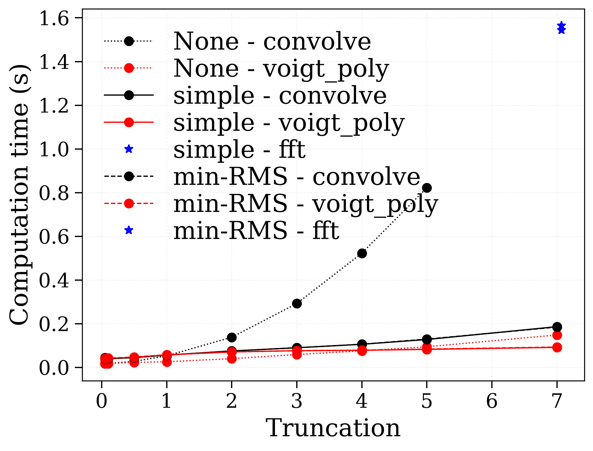
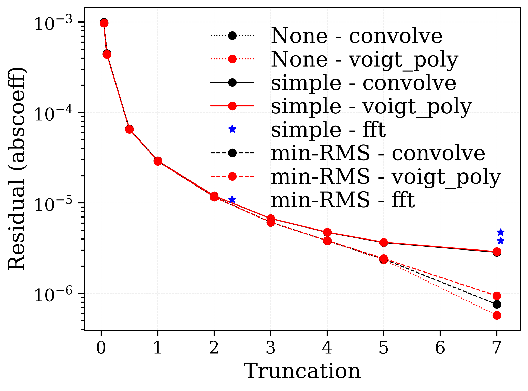
Truncation speeds up spectrum computation. This section shows its effect on
performance for several LDM optimizations and broadening methods. For all
methods, computation time increases roughly linearly with truncation width,
while the residual versus the reference decreases exponentially.
For any broadening method, a residual of diff/ref < 1e-6 is reachable with
both LDM methods, with computation times from 0.1 to 2 seconds. This is much
faster than 'LDM = None' with 'broadening_method = convolve', which takes
about 20 seconds.
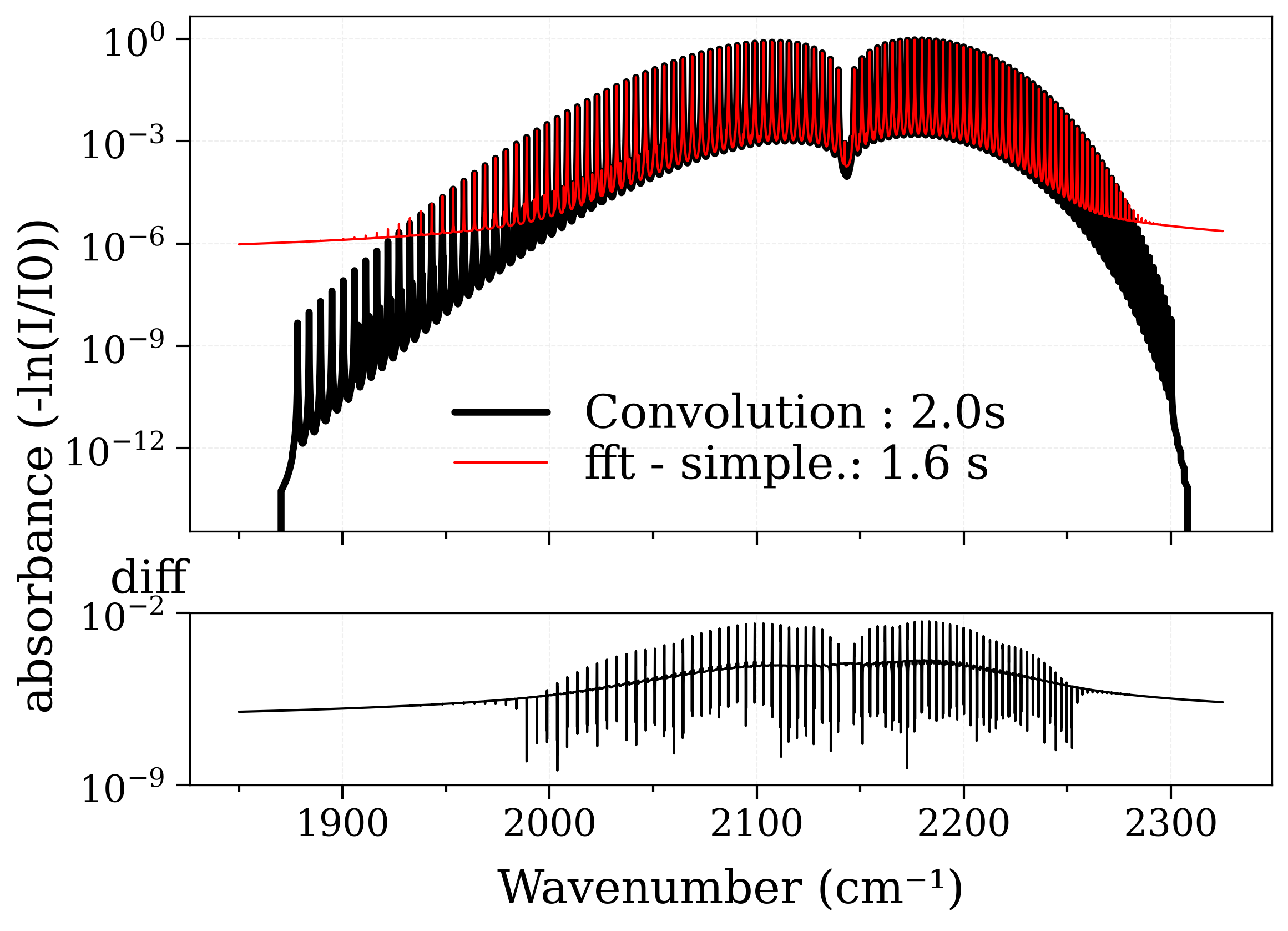
Note that the 'fft' method does not use truncation which explains the differences in the sides of the CO spectrum.
"""
s_ref = s_conv
import matplotlib.pyplot as plt
from tqdm import tqdm
from radis import get_residual
# Prepare the parameter grid for progress bar
trunc_values0 = [0.05, 0.1, 0.5, 1, 2, 3, 4, 5, 7]
LDM_values = [None, "simple", "min-RMS"]
method_values = ["convolve", "voigt_poly"]
conditions["verbose"] = False
total_iterations = (
sum(1 for trunc in trunc_values0 for LDM in LDM_values for method in method_values)
+ 2
)
progress = tqdm(total=total_iterations, desc="Processing")
results = {}
for LDM in LDM_values:
for method in method_values:
res_list, time_list = [], []
trunc_values = trunc_values0
if LDM is None and method == "convolve":
trunc_values = trunc_values0[:-1] # to avoid the longest computation
for trunc in trunc_values:
conditions["truncation"] = trunc
conditions["optimization"] = LDM
conditions["broadening_method"] = method
sf = SpectrumFactory(**conditions)
sf.fetch_databank(databank)
s = sf.eq_spectrum(Tgas=Tgas)
res_list.append(get_residual(s_ref, s, var="abscoeff"))
time_list.append(s.c["calculation_time"])
progress.update(1)
results[f"{LDM} - {method}"] = {
"trunc": trunc_values.copy(),
"residual": res_list,
"time": time_list,
}
## Add fft method (no truncation)
for LDM in ["simple", "min-RMS"]:
conditions["truncation"] = None
conditions["optimization"] = LDM
conditions["broadening_method"] = "fft"
sf = SpectrumFactory(**conditions)
sf.fetch_databank(databank)
s_fft = sf.eq_spectrum(Tgas=Tgas)
results[f"{LDM} - fft"] = {
"residual": get_residual(s_ref, s_fft, var="abscoeff"),
"time": s_fft.c["calculation_time"],
}
progress.update(1)
linestyles = {None: ":", "simple": "-", "min-RMS": "--"}
colors = {"convolve": "k", "voigt_poly": "r", "fft": "b"}
plt.figure("Time")
for LDM in LDM_values:
for method in method_values:
tag = f"{LDM} - {method}"
plt.plot(
results[tag]["trunc"],
results[tag]["time"],
f"{colors[method]}o",
linestyle=linestyles[LDM],
label=tag,
)
if LDM is not None:
tag = f"{LDM} - fft"
plt.plot(
max(trunc_values0) * 1.01,
results[tag]["time"],
f"{colors['fft']}*",
label=tag,
)
plt.xlabel("Truncation")
plt.ylabel("Computation time (s)")
plt.legend()
plt.figure("Residual")
for LDM in LDM_values:
for method, c in zip(method_values, colors):
tag = f"{LDM} - {method}"
plt.semilogy(
results[tag]["trunc"],
results[tag]["residual"],
f"{colors[method]}o",
linestyle=linestyles[LDM],
label=tag,
)
if LDM is not None:
tag = f"{LDM} - fft"
plt.plot(
max(trunc_values0) * 1.01,
results[tag]["residual"],
f"{colors['fft']}*",
label=tag,
)
plt.xlabel("Truncation")
plt.ylabel("Residual (abscoeff)")
plt.legend()
Processing:   0%|          | 0/56 [00:00<?, ?it/s]0.03s - Loaded database
/home/docs/checkouts/readthedocs.org/user_builds/radis/checkouts/latest/radis/misc/warning.py:445: CollisionalBroadeningWarning: Large error (57.8%) in pressure broadening. Increase broadening width / reduce wstep. Use .plot_broadening() to visualize each line broadening
  warnings.warn(WarningType(message))
0.03s - Loaded database
/home/docs/checkouts/readthedocs.org/user_builds/radis/checkouts/latest/radis/misc/warning.py:445: CollisionalBroadeningWarning: Large error (36.3%) in pressure broadening. Increase broadening width / reduce wstep. Use .plot_broadening() to visualize each line broadening
  warnings.warn(WarningType(message))

Processing:   4%|▎         | 2/56 [00:00<00:03, 16.91it/s]0.03s - Loaded database
/home/docs/checkouts/readthedocs.org/user_builds/radis/checkouts/latest/radis/misc/warning.py:445: CollisionalBroadeningWarning: Large error (8.1%) in pressure broadening. Increase broadening width / reduce wstep. Use .plot_broadening() to visualize each line broadening
  warnings.warn(WarningType(message))
0.03s - Loaded database
/home/docs/checkouts/readthedocs.org/user_builds/radis/checkouts/latest/radis/misc/warning.py:445: CollisionalBroadeningWarning: Large error (4.1%) in pressure broadening. Increase broadening width / reduce wstep. Use .plot_broadening() to visualize each line broadening
  warnings.warn(WarningType(message))

Processing:   7%|▋         | 4/56 [00:00<00:03, 14.02it/s]0.03s - Loaded database
/home/docs/checkouts/readthedocs.org/user_builds/radis/checkouts/latest/radis/misc/warning.py:445: CollisionalBroadeningWarning: Large error (2.0%) in pressure broadening. Increase broadening width / reduce wstep. Use .plot_broadening() to visualize each line broadening
  warnings.warn(WarningType(message))
0.03s - Loaded database
/home/docs/checkouts/readthedocs.org/user_builds/radis/checkouts/latest/radis/misc/warning.py:445: CollisionalBroadeningWarning: Large error (1.4%) in pressure broadening. Increase broadening width / reduce wstep. Use .plot_broadening() to visualize each line broadening
  warnings.warn(WarningType(message))

Processing:  11%|█         | 6/56 [00:00<00:07,  6.30it/s]0.03s - Loaded database
/home/docs/checkouts/readthedocs.org/user_builds/radis/checkouts/latest/radis/misc/warning.py:445: CollisionalBroadeningWarning: Large error (1.0%) in pressure broadening. Increase broadening width / reduce wstep. Use .plot_broadening() to visualize each line broadening
  warnings.warn(WarningType(message))

Processing:  12%|█▎        | 7/56 [00:01<00:12,  3.82it/s]0.03s - Loaded database

Processing:  14%|█▍        | 8/56 [00:02<00:20,  2.40it/s]0.03s - Loaded database
0.03s - Loaded database

Processing:  18%|█▊        | 10/56 [00:02<00:12,  3.78it/s]0.03s - Loaded database
0.03s - Loaded database

Processing:  21%|██▏       | 12/56 [00:02<00:08,  5.29it/s]0.03s - Loaded database
0.03s - Loaded database

Processing:  25%|██▌       | 14/56 [00:02<00:06,  6.48it/s]0.03s - Loaded database
0.03s - Loaded database

Processing:  29%|██▊       | 16/56 [00:02<00:05,  6.83it/s]0.03s - Loaded database

Processing:  30%|███       | 17/56 [00:03<00:05,  6.50it/s]0.03s - Loaded database
0.03s - Loaded database

Processing:  34%|███▍      | 19/56 [00:03<00:04,  7.83it/s]0.03s - Loaded database
0.03s - Loaded database

Processing:  38%|███▊      | 21/56 [00:03<00:04,  8.58it/s]0.03s - Loaded database

Processing:  39%|███▉      | 22/56 [00:03<00:03,  8.57it/s]0.03s - Loaded database

Processing:  41%|████      | 23/56 [00:03<00:03,  8.33it/s]0.03s - Loaded database

Processing:  43%|████▎     | 24/56 [00:03<00:04,  7.88it/s]0.03s - Loaded database

Processing:  45%|████▍     | 25/56 [00:04<00:04,  7.25it/s]0.03s - Loaded database

Processing:  46%|████▋     | 26/56 [00:04<00:04,  6.19it/s]0.03s - Loaded database
0.03s - Loaded database

Processing:  50%|█████     | 28/56 [00:04<00:03,  7.83it/s]0.03s - Loaded database
0.03s - Loaded database

Processing:  54%|█████▎    | 30/56 [00:04<00:02,  8.70it/s]0.03s - Loaded database

Processing:  55%|█████▌    | 31/56 [00:04<00:02,  8.73it/s]0.03s - Loaded database

Processing:  57%|█████▋    | 32/56 [00:04<00:02,  8.65it/s]0.03s - Loaded database

Processing:  59%|█████▉    | 33/56 [00:04<00:02,  8.56it/s]0.03s - Loaded database

Processing:  61%|██████    | 34/56 [00:05<00:02,  8.40it/s]0.03s - Loaded database

Processing:  62%|██████▎   | 35/56 [00:05<00:02,  8.10it/s]0.03s - Loaded database
0.03s - Loaded database

Processing:  66%|██████▌   | 37/56 [00:05<00:01,  9.53it/s]0.03s - Loaded database
0.03s - Loaded database

Processing:  70%|██████▉   | 39/56 [00:05<00:01,  9.94it/s]0.03s - Loaded database

Processing:  71%|███████▏  | 40/56 [00:05<00:01,  9.61it/s]0.03s - Loaded database

Processing:  73%|███████▎  | 41/56 [00:05<00:01,  9.03it/s]0.03s - Loaded database

Processing:  75%|███████▌  | 42/56 [00:05<00:01,  8.32it/s]0.03s - Loaded database

Processing:  77%|███████▋  | 43/56 [00:06<00:01,  7.49it/s]0.03s - Loaded database

Processing:  79%|███████▊  | 44/56 [00:06<00:01,  6.29it/s]0.03s - Loaded database
0.03s - Loaded database

Processing:  82%|████████▏ | 46/56 [00:06<00:01,  7.97it/s]0.03s - Loaded database
0.03s - Loaded database

Processing:  86%|████████▌ | 48/56 [00:06<00:00,  8.81it/s]0.03s - Loaded database

Processing:  88%|████████▊ | 49/56 [00:06<00:00,  8.83it/s]0.03s - Loaded database

Processing:  89%|████████▉ | 50/56 [00:06<00:00,  8.76it/s]0.03s - Loaded database

Processing:  91%|█████████ | 51/56 [00:07<00:00,  8.65it/s]0.03s - Loaded database

Processing:  93%|█████████▎| 52/56 [00:07<00:00,  8.49it/s]0.03s - Loaded database

Processing:  95%|█████████▍| 53/56 [00:07<00:00,  8.18it/s]0.03s - Loaded database

Processing:  96%|█████████▋| 54/56 [00:08<00:01,  1.85it/s]0.03s - Loaded database

Processing:  98%|█████████▊| 55/56 [00:10<00:00,  1.17it/s]
<matplotlib.legend.Legend object at 0x71bd6c2156a0>
Total running time of the script: (0 minutes 32.974 seconds)