


radis.lbl package
Submodules
- radis.lbl.bands module
- Routine Listing
BandFactoryBandFactory.NwGBandFactory.NwLBandFactory.SpecDatabaseBandFactory.autoretrievedatabaseBandFactory.autoupdatedatabaseBandFactory.cond_unitsBandFactory.databaseBandFactory.dataframe_engineBandFactory.dataframe_typeBandFactory.df0BandFactory.df1BandFactory.eq_bands()BandFactory.get_band()BandFactory.get_band_list()BandFactory.get_bands_weight()BandFactory.inputBandFactory.input_wunitBandFactory.interactive_paramsBandFactory.levelsBandFactory.levelspathBandFactory.min_widthBandFactory.miscBandFactory.molparamBandFactory.non_eq_bands()BandFactory.paramsBandFactory.parsumBandFactory.parsum_calcBandFactory.parsum_tabBandFactory.profilerBandFactory.reftrackerBandFactory.save_memoryBandFactory.truncationBandFactory.unitsBandFactory.verboseBandFactory.warningsBandFactory.wavenumberBandFactory.wavenumber_calcBandFactory.wbroad_centeredBandFactory.woutrange
add_bands()docstring_parameter()
- radis.lbl.base module
- Summary
- Routine Listing
BaseFactoryBaseFactory.NwGBaseFactory.NwLBaseFactory.Qgas()BaseFactory.Qneq()BaseFactory.Qneq_Qvib_Qrotu_Qrotl()BaseFactory.Qref_Qgas_ratio()BaseFactory.SpecDatabaseBaseFactory.assert_no_nan()BaseFactory.autoretrievedatabaseBaseFactory.autoupdatedatabaseBaseFactory.calc_S0()BaseFactory.calc_einstein_coefficients()BaseFactory.calc_emission_integral()BaseFactory.calc_lineshift()BaseFactory.calc_linestrength_eq()BaseFactory.calc_linestrength_noneq()BaseFactory.calc_populations_eq()BaseFactory.calc_populations_noneq()BaseFactory.calc_weighted_trans_moment()BaseFactory.cond_unitsBaseFactory.cond_units0BaseFactory.databaseBaseFactory.dataframe_engineBaseFactory.dataframe_typeBaseFactory.df0BaseFactory.df1BaseFactory.get_energy_levels()BaseFactory.get_lines()BaseFactory.get_lines_abundance()BaseFactory.get_molar_mass()BaseFactory.get_populations()BaseFactory.inputBaseFactory.input_wunitBaseFactory.interactive_paramsBaseFactory.levelsBaseFactory.levelspathBaseFactory.min_widthBaseFactory.miscBaseFactory.molparamBaseFactory.paramsBaseFactory.parsumBaseFactory.parsum_calcBaseFactory.parsum_tabBaseFactory.plot_hist()BaseFactory.plot_linestrength_hist()BaseFactory.plot_populations()BaseFactory.print_conditions()BaseFactory.profilerBaseFactory.reftrackerBaseFactory.save_memoryBaseFactory.truncationBaseFactory.unitsBaseFactory.units0BaseFactory.verboseBaseFactory.warningsBaseFactory.wavenumberBaseFactory.wavenumber_calcBaseFactory.wbroad_centeredBaseFactory.woutrange
get_wavenumber_range()linestrength_from_Einstein()
- radis.lbl.broadening module
- Summary
- Routine Listing
BroadenFactoryBroadenFactory.NwGBroadenFactory.NwLBroadenFactory.SpecDatabaseBroadenFactory.autoretrievedatabaseBroadenFactory.autoupdatedatabaseBroadenFactory.calculate_pseudo_continuum()BroadenFactory.cond_unitsBroadenFactory.databaseBroadenFactory.dataframe_engineBroadenFactory.dataframe_typeBroadenFactory.df0BroadenFactory.df1BroadenFactory.inputBroadenFactory.input_wunitBroadenFactory.interactive_paramsBroadenFactory.levelsBroadenFactory.levelspathBroadenFactory.min_widthBroadenFactory.miscBroadenFactory.molparamBroadenFactory.paramsBroadenFactory.parsumBroadenFactory.parsum_calcBroadenFactory.parsum_tabBroadenFactory.plot_broadening()BroadenFactory.profilerBroadenFactory.reftrackerBroadenFactory.save_memoryBroadenFactory.truncationBroadenFactory.unitsBroadenFactory.verboseBroadenFactory.warningsBroadenFactory.wavenumberBroadenFactory.wavenumber_calcBroadenFactory.wbroad_centeredBroadenFactory.woutrange
doppler_broadening_HWHM()gamma_vald3()gaussian_FT()gaussian_lineshape()lorentzian_FT()lorentzian_lineshape()olivero_1977()pressure_broadening_HWHM()project_lines_on_grid()project_lines_on_grid_noneq()voigt_FT()voigt_broadening_HWHM()voigt_lineshape()whiting1968()
- radis.lbl.calc module
- radis.lbl.factory module
- Routine Listing
SpectrumFactorySpectrumFactory.NwGSpectrumFactory.NwLSpectrumFactory.SpecDatabaseSpectrumFactory.autoretrievedatabaseSpectrumFactory.autoupdatedatabaseSpectrumFactory.cond_unitsSpectrumFactory.databaseSpectrumFactory.dataframe_engineSpectrumFactory.dataframe_typeSpectrumFactory.df0SpectrumFactory.df1SpectrumFactory.eq_spectrum()SpectrumFactory.eq_spectrum_gpu()SpectrumFactory.eq_spectrum_gpu_interactive()SpectrumFactory.fit_legacy()SpectrumFactory.generate_perf_profile()SpectrumFactory.inputSpectrumFactory.input_wunitSpectrumFactory.interactive_paramsSpectrumFactory.levelsSpectrumFactory.levelspathSpectrumFactory.min_widthSpectrumFactory.miscSpectrumFactory.molparamSpectrumFactory.non_eq_spectrum()SpectrumFactory.optically_thin_power()SpectrumFactory.paramsSpectrumFactory.parsumSpectrumFactory.parsum_calcSpectrumFactory.parsum_tabSpectrumFactory.predict_time()SpectrumFactory.print_perf_profile()SpectrumFactory.profilerSpectrumFactory.reftrackerSpectrumFactory.save_memorySpectrumFactory.truncationSpectrumFactory.unitsSpectrumFactory.verboseSpectrumFactory.warningsSpectrumFactory.wavenumberSpectrumFactory.wavenumber_calcSpectrumFactory.wbroad_centeredSpectrumFactory.woutrange
- radis.lbl.labels module
- radis.lbl.loader module
- Summary
- Routine Listings
ConditionDictDatabankLoaderDatabankLoader.NwGDatabankLoader.NwLDatabankLoader.SpecDatabaseDatabankLoader.autoretrievedatabaseDatabankLoader.autoupdatedatabaseDatabankLoader.columns_list_to_load()DatabankLoader.cond_unitsDatabankLoader.databaseDatabankLoader.dataframe_engineDatabankLoader.dataframe_typeDatabankLoader.df0DatabankLoader.df1DatabankLoader.fetch_databank()DatabankLoader.get_abundance()DatabankLoader.get_conditions()DatabankLoader.get_partition_function_calculator()DatabankLoader.get_partition_function_interpolator()DatabankLoader.get_partition_function_molecule()DatabankLoader.init_databank()DatabankLoader.init_database()DatabankLoader.inputDatabankLoader.input_wunitDatabankLoader.interactive_paramsDatabankLoader.levelsDatabankLoader.levelspathDatabankLoader.load_databank()DatabankLoader.min_widthDatabankLoader.miscDatabankLoader.molparamDatabankLoader.paramsDatabankLoader.parsumDatabankLoader.parsum_calcDatabankLoader.parsum_tabDatabankLoader.profilerDatabankLoader.reftrackerDatabankLoader.save_memoryDatabankLoader.set_abundance()DatabankLoader.set_atomic_partition_functions()DatabankLoader.truncationDatabankLoader.unitsDatabankLoader.verboseDatabankLoader.warn()DatabankLoader.warningsDatabankLoader.wavenumberDatabankLoader.wavenumber_calcDatabankLoader.wbroad_centeredDatabankLoader.woutrange
InputInput.TelecInput.TgasInput.TrefInput.TrotInput.TvibInput.isatomInput.isneutralInput.isotopeInput.mediumInput.mole_fractionInput.moleculeInput.overpopulationInput.path_lengthInput.pfsourceInput.potential_loweringInput.pressureInput.rot_distributionInput.self_absorptionInput.speciesInput.stateInput.vib_distributionInput.wavelength_maxInput.wavelength_minInput.wavenum_maxInput.wavenum_min
KNOWN_DBFORMATKNOWN_LVLFORMATKNOWN_PARFUNCFORMATMiscParamsMiscParams.add_at_usedMiscParams.chunksizeMiscParams.export_linesMiscParams.export_populationsMiscParams.export_rovib_fractionMiscParams.load_energiesMiscParams.memory_mapping_engineMiscParams.total_linesMiscParams.warning_broadening_thresholdMiscParams.warning_linestrength_cutoffMiscParams.zero_padding
ParametersParameters.broadening_methodParameters.chunksizeParameters.cutoffParameters.db_use_cachedParameters.dbformatParameters.dbpathParameters.diluentParameters.dxGParameters.dxLParameters.export_linesParameters.export_populationsParameters.folding_threshParameters.include_neighbouring_linesParameters.lbfuncParameters.levelsfmtParameters.lvl_use_cachedParameters.neighbour_linesParameters.optimizationParameters.parfuncpathParameters.parsum_modeParameters.pseudo_continuum_thresholdParameters.sparse_ldmParameters.truncationParameters.warning_broadening_thresholdParameters.warning_linestrength_cutoffParameters.wavenum_max_calcParameters.wavenum_min_calcParameters.waveunitParameters.wstep
broadening_coeffdf_metadatadrop_all_but_thesedrop_auto_columns_for_dbformatdrop_auto_columns_for_levelsfmtformat_paths()required_non_eq
- radis.lbl.overp module
- Summary
LevelsListLevelsList.E_bandsLevelsList.QrefLevelsList.Qvib_refLevelsList.Trot_refLevelsList.Tvib_refLevelsList.bandsLevelsList.bands_refLevelsList.copy_linesLevelsList.cum_weightLevelsList.eq_spectrum()LevelsList.levelsfmtLevelsList.lvl_indexLevelsList.mole_fraction_refLevelsList.non_eq_spectrum()LevelsList.parfuncLevelsList.path_length_refLevelsList.plot_vib_populations()LevelsList.sorted_bandsLevelsList.verboseLevelsList.vib_distribution_refLevelsList.vib_levels
rescale_updown_levels()
Module contents
Core of the line-by-line calculations
- class LevelsList(parfunc, bands, levelsfmt, sortby='Ei', copy_lines=False, verbose=True)[source]
Bases:
objectA class to generate a Spectrum from a list of precalculated bands at a given reference temperature.
Warning
only valid under optically thin conditions!!
- eq_spectrum(Tgas, overpopulation=None, mole_fraction=None, path_length=None, save_rescaled_bands=False)[source]
See
eq_spectrum()Warning
only valid under optically thin conditions!!
- Parameters:
… same as usually. If None, then the reference value (used to
calculate bands) is used
- Other Parameters:
save_rescaled_bands (boolean) – save updated bands. Take some time as it requires rescaling all bands individually (which is only done on the MergedSlabs usually) Default
False
- non_eq_spectrum(Tvib=None, Trot=None, Ttrans=None, vib_distribution='boltzmann', overpopulation=None, mole_fraction=None, path_length=None, save_rescaled_bands=False)[source]
-
Warning
only valid under optically thin conditions!!
- Parameters:
… same as usually. If None, then the reference value (used to
calculate bands) is used
- Other Parameters:
save_rescaled_bands (boolean) – save updated bands. Take some time as it requires rescaling all bands individually (which is only done on the MergedSlabs usually) Default
False
Notes
Implementation:
Generation of a new spectrum is done by recombination of the precalculated bands with
- plot_vib_populations(nfig=None, **kwargs)[source]
Plot current distribution of vibrational levels.
By constructions populations are shown as divided by the state degeneracy, i.e, g = gv * (2J+1) * gi * gs
- Parameters:
nfig (str, int) – name of Figure to plot on
kwargs (**dict) – arguments are forwarded to plot()
- class SpectrumFactory(wmin=None, wmax=None, wunit=cm - 1, wavenum_min=None, wavenum_max=None, wavelength_min=None, wavelength_max=None, Tref=296, pressure=1.01325, mole_fraction=1, path_length=1, wstep=0.01, isotope='all', medium='air', truncation=50, neighbour_lines=0, pseudo_continuum_threshold=0, self_absorption=True, chunksize=None, optimization='simple', folding_thresh=1e-06, zero_padding=-1, broadening_method='voigt', cutoff=0, parsum_mode='full summation', verbose=True, warnings=True, species=None, save_memory=False, export_populations=None, export_lines=False, gpu_backend=None, diluent=None, lbfunc=None, potential_lowering=None, pfsource='default', **kwargs)[source]
Bases:
BandFactoryA class to put together all functions related to loading CDSD and HITRAN databases, calculating the broadenings, and summing over all the lines.
- Parameters:
wmin, wmax (
floatorQuantity) – a hybrid parameter which can stand for minimum (maximum) wavenumber or minimum (maximum) wavelength depending upon the unit accompanying it. If dimensionless,wunitis considered as the accompanying unit.wunit (
'nm','cm-1') – the unit accompanying wmin and wmax. Can only be passed with wmin and wmax. Default is"cm-1".wavenum_min, wavenum_max (
float(cm^-1)orQuantity) – minimum (maximum) wavenumber to be processed in \(cm^{-1}\). use astropy.units to specify arbitrary inverse-length units.wavelength_min, wavelength_max (
float(nm)orQuantity) – minimum (maximum) wavelength to be processed in \(nm\). This wavelength can be in'air'or'vacuum'depending on the value of the parametermedium=. use astropy.units to specify arbitrary length units.pressure (
float(bar)orQuantity) – partial pressure of gas in bar. Default1.01325(1 atm). use astropy.units to specify arbitrary pressure units. For example,1013.25 * u.mbar.mole_fraction (
float[ 0 - 1]) – species mole fraction. Default1. Note that the rest of the gas is considered to be air for collisional broadening.path_length (
float(cm)orQuantity) – path length in cm. Default1. use astropy.units to specify arbitrary length units.species (
int,str, orNone) –- For molecules:
molecule id (HITRAN format) or name. If
None, the molecule can be inferred from the database files being loaded. See the list of supported molecules inMOLECULES_LIST_EQUILIBRIUMandMOLECULES_LIST_NONEQUILIBRIUM.- For atoms:
The positive or neutral atomic species (negative ions aren’t supported). It may be given in spectroscopic notation or any form that can be converted by
to_conventional_name()
Default
None.isotope (
int,list,strof the form'1,2', or'all') – isotope idFor molecules, this is the isotopologue ID (sorted by relative density: (eg: 1: CO2-626, 2: CO2-636 for CO2) - see [HITRAN-2020] documentation for isotope list for all species.
For atoms, use the isotope number of the isotope (the total number of protons and neutrons in the nucleus) - use 0 to select rows where the isotope is unspecified, in which case the standard atomic weight from the
periodictablemodule is used when mass is required.If
'all', all isotopes in database are used (this may result in larger computation times!).Default
'all'medium (
'air','vacuum') – propagating medium when giving inputs with'wavenum_min','wavenum_max'. Does not change anything when giving inputs in wavenumber. Default'air'diluent (
strordictionary) – can be a string of a single diluent or a dictionary containing diluent name as key and its mole_fraction as value.If left unspecified, it defaults to
'air'for molecules and atomic hydrogen ‘H’ for atoms.For free electrons, use the symbol ‘e-’. Currently, only H, H2, H2, and e- are supported for atoms - any other diluents have no effect besides diluting the mole fractions of the other constituents.
- Other Parameters:
Tref (K) – Reference temperature for calculations (linestrength temperature correction). HITRAN database uses 296 Kelvin. Default 296 K
self_absorption (boolean) – Compute self absorption. If
False, spectra are optically thin. DefaultTrue.truncation (float (\(cm^{-1}\))) – Half-width over which to compute the lineshape, i.e. lines are truncated on each side after
truncation(\(cm^{-1}\)) from the line center. IfNone, use no truncation (lineshapes spread on the full spectral range). Default is50\(cm^{-1}\)Note
Large values (>
50) can induce a performance drop (computation of lineshape typically scale as \(~truncation ^2\) ). The default50was chosen to maintain a good accuracy, and still exhibit the sub-Lorentzian behavior of most lines far (few hundreds \(cm^{-1}\)) from the line center.neighbour_lines (float (\(cm^{-1}\))) – The calculated spectral range is increased (by
neighbour_linescm-1 on each side) to take into account overlaps from out-of-range lines. Default is0\(cm^{-1}\).wstep (float (cm-1) or
'auto') – Resolution of wavenumber grid. Default0.01cm-1. If'auto', it is ensured that there are slightly more points for each linewidth than the value of"GRIDPOINTS_PER_LINEWIDTH_WARN_THRESHOLD"inradis.config(~/radis.json)Note
wstep = ‘auto’ is optimized for performances while ensuring accuracy, but is still experimental in 0.9.30. Feedback welcome!
cutoff (float (~ unit of Linestrength: cm-1/(#.cm-2))) – discard linestrengths that are lower that this, to reduce calculation times.
1e-27is what is generally used to generate databases such as CDSD. If0, no cutoff. Default1e-27.parsum_mode (‘full summation’, ‘tabulation’) – how to compute partition functions, at nonequilibrium or when partition function are not already tabulated.
'full summation': sums over all (potentially millions) of rovibrational levels.'tabulation': builds an on-the-fly tabulation of rovibrational levels (500 - 4000x faster and usually accurate within 0.1%). Defaultfull summation'Note
parsum_mode= ‘tabulation’ is new in 0.9.30, and makes nonequilibrium calculations of small spectra extremely fast. Will become the default after 0.9.31.
pseudo_continuum_threshold (float) – if not
0, first calculate a rough approximation of the spectrum, then moves all lines whose linestrength intensity is less than this threshold of the maximum in a semi-continuum. Values above 0.01 can yield significant errors, mostly in highly populated areas. 80% of the lines can typically be moved in a continuum, resulting in 5 times faster spectra. If0, no semi-continuum is used. Default0.save_memory (boolean) – if
True, removes databases calculated by intermediate functions (for instance, delete the full database once the linestrength cutoff criteria was applied). This saves some memory but requires to reload the database and recalculate the linestrength for each new parameter. DefaultFalse.export_populations (
'vib','rovib',None) – if not None, store populations in Spectrum. Either store vibrational populations (‘vib’) or rovibrational populations (‘rovib’). DefaultNoneexport_lines (boolean) – if
True, saves details of all calculated lines in Spectrum. This is necessary to later useline_survey(), but can take some space. DefaultFalse.chunksize (int, or
None) – Splits the lines database in several chunks during calculation, else the multiplication of lines over all spectral range takes too much memory and slows the system down. Chunksize let you change the default chunk size. IfNone, all lines are processed directly. Usually faster but can create memory problems. DefaultNoneoptimization (
"simple","min-RMS",None) – If either"simple"or"min-RMS"LDM optimization for lineshape calculation is used: -"min-RMS": weights optimized by analytical minimization of the RMS-error (See: [Spectral-Synthesis-Algorithm]) -"simple": weights equal to their relative position in the gridIf
None, no lineshape interpolation is performed and the lineshape of all lines is calculated.Refer to [Spectral-Synthesis-Algorithm] for more explanation on the LDM method for lineshape interpolation.
Default
"min-RMS"folding_thresh (float) – Folding is a correction procedure that is applied when the lineshape is calculated with the
fftbroadening method and the linewidth is comparable towstep, that prevents sinc(v) modulation of the lineshape. Folding continues until the lineshape intensity is belowfolding_threshold. Setting to 1 or higher effectively disables folding correction.Range: 0.0 < folding_thresh <= 1.0 Default: 1e-6
zero_padding (int) – Zero padding is used in conjunction with the
fftbroadening method to prevent circular convolution at the cost of performance. When set to -1, padding is set equal to the spectrum length, which guarantees a linear convolution.Range: 0 <= zero_padding <= len(w), or zero_padding = -1 Default: -1
broadening_method (
"voigt","convolve","fft") – Calculates broadening with a direct voigt approximation (‘voigt’) or by convoluting independently calculated Doppler and collisional broadening (‘convolve’). First is much faster, 2nd can be used to compare results. This SpectrumFactory parameter can be manually adjusted a posteriori with:sf = SpectrumFactory(...) sf.params.broadening_method = 'voigt'
Fast fourier transform
'fft'is only available if using the LDM lineshape calculationoptimization. Because the LDM convolves all lines at the same time, and thus operates on large arrays,'fft'becomes more appropriate than convolutions in real space ('voigt','convolve')By default, use
"fft"for anyoptimization, and"voigt"if optimization isNone.warnings (bool, or one of
['warn', 'error', 'ignore'], dict) – If one of['warn', 'error', 'ignore'], set the default behaviour for all warnings. Can also be a dictionary to set specific warnings only. Example:warnings = {'MissingSelfBroadeningWarning':'ignore', 'NegativeEnergiesWarning':'ignore', 'HighTemperatureWarning':'ignore'}
See
default_warning_statusfor more information.verbose (boolean, or int) – If
False, stays quiet. IfTrue, tells what is going on. If>=2, gives more detailed messages (for instance, details of calculation times). DefaultTrue.lbfunc (callable) –
- An alternative function to be used instead of the default in calculating Lorentzian broadening, which receives the following:
df: the dataframeself.df1containing the quantities used for calculating the spectrumpressure_atm:self.pressurein units of atmospheric pressure (1.01325 bar)mole_fraction:self.input.mole_fraction, the mole fraction of the species for which the spectrum is being calculatedTgas:self.input.Tgas, gas temperature in KTref:self.input.Tref, reference temperature for calculations in Kdiluent:self._diluent, the dictionary of diluents giving the mole fraction of eachdiluent_broadening_coeff: a dictionary of the broadening coefficients for each diluentisneutral: When calculating the spectrum of an atomic species, whether or not it is neutral (alwaysNonefor molecules)
- Returns:
gamma_lb,shift- The total Lorentzian HWHM [\(cm^{-1}\)], and the shift [\(cm^{-1}\)] to be subtracted from the wavenumber array to account for lineshift. If setting the lineshift here is not desired, the 2nd return object can be anything for whichbool(shift)==FalselikeNone. gamma_lb must be array-like but can also be a vaex expression if the dataframe type is vaex.
If unspecified, the broadening is handled by default by
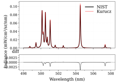
gamma_vald3()for atoms when using the Kurucz databank, andpressure_broadening_HWHM()for molecules.For the NIST databank, the
lbfuncparameter is compulsory as NIST doesn’t provide broadening parameters.pfsource (
string) – The source for the partition function tables for an interpolator or energy level tables for a calculator. Sources implemented so far are ‘barklem’ and ‘kurucz’ for the former, and ‘nist’ for the latter. ‘default’ is currently ‘nist’. Thepfsourcecan be changed post-initialisation using theset_atomic_partition_functions()method. See the provided example for more details.potential_lowering (float (cm-1/Zeff**2)) – The value of potential lowering, only relevant when
pfsourceis ‘kurucz’ as it depends on both temperature and potential lowering. Can be changed on the fly by settingsf.input.potential_lowering. Allowed values are typically: -500, -1000, -2000, -4000, -8000, -16000, -32000. Again, see the provided example for more details.
Examples
An example using
SpectrumFactory,load_databank(), theSpectrummethods, andunitsfrom radis import SpectrumFactory from astropy import units as u sf = SpectrumFactory(wavelength_min=4165 * u.nm, wavelength_max=4200 * u.nm, isotope='1,2', truncation=10, # cm-1 optimization=None, medium='vacuum', verbose=1, # more for more details ) sf.load_databank('HITRAN-CO2-TEST') # predefined in ~/radis.json s = sf.eq_spectrum(Tgas=300 * u.K, path_length=1 * u.cm) s.rescale_path_length(0.01) # cm s.plot('radiance_noslit', Iunit='µW/cm2/sr/nm')
Refer to the online Examples for more cases.
Examples using
radis.SpectrumFactory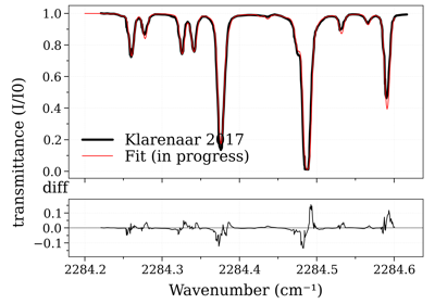
Legacy #2: non-equilibrium CO2 (Tvib_12, Tvib_3, Trot)
Legacy #2: non-equilibrium CO2 (Tvib_12, Tvib_3, Trot)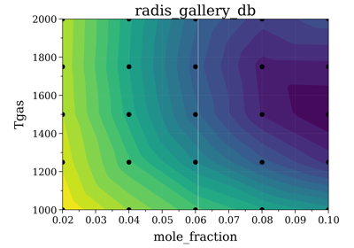
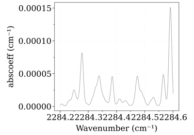
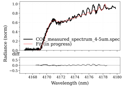
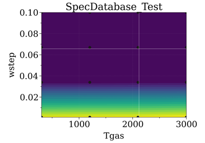
Example #7: Database fitting using SpecDatabase.fit_spectrum
Example #7: Database fitting using SpecDatabase.fit_spectrumNotes
digraph inheritanceb7d785f131 { bgcolor=transparent; rankdir=LR; size="8.0, 12.0"; "BandFactory" [URL="radis.lbl.bands.html#radis.lbl.bands.BandFactory",fillcolor=white,fontname="Vera Sans, DejaVu Sans, Liberation Sans, Arial, Helvetica, sans",fontsize=10,height=0.25,shape=box,style="setlinewidth(0.5),filled",target="_top",tooltip="See Also"]; "BroadenFactory" -> "BandFactory" [arrowsize=0.5,style="setlinewidth(0.5)"]; "BaseFactory" [URL="radis.lbl.base.html#radis.lbl.base.BaseFactory",fillcolor=white,fontname="Vera Sans, DejaVu Sans, Liberation Sans, Arial, Helvetica, sans",fontsize=10,height=0.25,shape=box,style="setlinewidth(0.5),filled",target="_top"]; "DatabankLoader" -> "BaseFactory" [arrowsize=0.5,style="setlinewidth(0.5)"]; "BroadenFactory" [URL="radis.lbl.broadening.html#radis.lbl.broadening.BroadenFactory",fillcolor=white,fontname="Vera Sans, DejaVu Sans, Liberation Sans, Arial, Helvetica, sans",fontsize=10,height=0.25,shape=box,style="setlinewidth(0.5),filled",target="_top",tooltip="A class that holds all broadening methods."]; "BaseFactory" -> "BroadenFactory" [arrowsize=0.5,style="setlinewidth(0.5)"]; "DatabankLoader" [URL="radis.lbl.loader.html#radis.lbl.loader.DatabankLoader",fillcolor=white,fontname="Vera Sans, DejaVu Sans, Liberation Sans, Arial, Helvetica, sans",fontsize=10,height=0.25,shape=box,style="setlinewidth(0.5),filled",target="_top",tooltip=".. inheritance-diagram:: radis.lbl.factory.SpectrumFactory"]; "SpectrumFactory" [URL="radis.lbl.factory.html#radis.lbl.factory.SpectrumFactory",fillcolor=white,fontname="Vera Sans, DejaVu Sans, Liberation Sans, Arial, Helvetica, sans",fontsize=10,height=0.25,shape=box,style="setlinewidth(0.5),filled",target="_top",tooltip="A class to put together all functions related to loading CDSD and HITRAN"]; "BandFactory" -> "SpectrumFactory" [arrowsize=0.5,style="setlinewidth(0.5)"]; }High-level wrapper to SpectrumFactory:
Main Methods:
For advanced use:
Inputs and parameters can be accessed a posteriori with :
input: physical inputparams: computational parametersmisc: miscellaneous parameters (don’t change output)
References
See also
- df0[source]
initial line database after loading. If for any reason, you want to manipulate the line database manually (for instance, keeping only lines emitting by a particular level), you need to access the
df0attribute ofSpectrumFactory.Warning
never overwrite the
df0attribute, else some metadata may be lost in the process. Only use inplace operations. If reducing the number of lines, add a df0.reset_index()For instance:
from radis import SpectrumFactory
sf = SpectrumFactory(
    wavenum_min= 2150.4,
    wavenum_max=2151.4,
    pressure=1,
    isotope=1)
sf.load_databank('HITRAN-CO-TEST')
sf.df0.drop(sf.df0[sf.df0.vu!=1].index, inplace=True)   # keep lines emitted by v'=1 only
sf.eq_spectrum(Tgas=3000, name='vu=1').plot()
df0contains the lines as they are loaded from the database.df1is generated during the spectrum calculation, after the line database reduction steps, population calculation, and scaling of intensity and broadening parameters with the calculated conditions.See also
df1- Type:
pd.DataFrame
- df1[source]
line database, scaled with populations + linestrength cutoff Never edit manually. See all comments about
df0See also
df0- Type:
pd.DataFrame
- eq_spectrum(Tgas, mole_fraction=None, path_length=None, diluent=None, pressure=None, name=None) Spectrum[source]
Generate a spectrum at equilibrium.
- Parameters:
Tgas (float or
Quantity) – Gas temperature (K)mole_fraction (float) – database species mole fraction. If None, Factory mole fraction is used.
diluent (str or dictionary) – can be a string of a single diluent or a dictionary containing diluent name as key and its mole_fraction as value
path_length (float or
Quantity) – slab size (cm). IfNone, the default Factorypath_lengthis used.pressure (float or
Quantity) – pressure (bar). IfNone, the default Factorypressureis used.name (str) – output Spectrum name (useful in batch)
- Returns:
s –
Returns a
Spectrumobject- Return type:
Examples
- ::
from radis import SpectrumFactory sf = SpectrumFactory( wavenum_min=2900, wavenum_max=3200, molecule=”OH”, wstep=0.1, ) sf.fetch_databank(“hitemp”)
s1 = sf.eq_spectrum(Tgas=300, path_length=1, pressure=0.1) s2 = sf.eq_spectrum(Tgas=500, path_length=1, pressure=0.1)
References
See also
- eq_spectrum_gpu(Tgas, mole_fraction=None, diluent=None, path_length=None, pressure=None, name=None, backend='vulkan', device_id=0, exit_gpu=False, verbose=None) Spectrum[source]
Generate a spectrum at equilibrium with calculation of lineshapes and broadening done on the GPU.
- Parameters:
Tgas (float or
Quantity) – Gas temperature (K)mole_fraction (float) – database species mole fraction. If None, Factory mole fraction is used.
path_length (float or
Quantity) – slab size (cm). IfNone, the default Factorypath_lengthis used.pressure (float or
Quantity) – pressure (bar). IfNone, the default Factorypressureis used.name (str) – output Spectrum name (useful in batch)
- Other Parameters:
device_id (int, str) – Select the GPU device. If
int, specifies the device index, which is printed for convenience during GPU initialization with backend=’vulkan’ (default). Ifstr, return the first device that includes the specified string (case-insensitive). If not found, return the device at index 0. default = 0exit_gpu (bool) – Specifies whether the GPU app should be exited after producing the spectrum. Usually this is undesirable, because the GPU computations start to benefit after the first spectrum is produced by calling s.recalc_gpu(). See also
recalc_gpu()default = Falsebackend (str) – Since version 0.16, only
'vulkan'backend is supported. In previous versions,'gpu-cuda'and'cpu-cuda'were available to switch to a CUDA backend, but this has been deprecated in favor of the Vulkan backend... warning:: – The
backendparameter is deprecated. Only the Vulkan backend is supported.
- Returns:
s – Returns a
SpectrumobjectUse the
get()method to get something among['radiance', 'radiance_noslit', 'absorbance', etc...]Or directly the
plot()method to plot it. See [1]_ to get an overview of all Spectrum methods- Return type:
Examples
Examples using
radis.lbl.SpectrumFactory.eq_spectrum_gpu¶See also
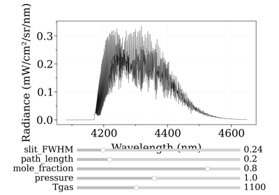
- eq_spectrum_gpu_interactive(var='transmittance', slit_function=0.0, mpl_backend='', plotkwargs={}, *vargs, **kwargs) Spectrum[source]
- Parameters:
var (TYPE, optional) – DESCRIPTION. The default is “transmittance”.
slit_function (TYPE, optional) – DESCRIPTION. The default is 0.0.
*vargs (TYPE) – arguments forwarded to
eq_spectrum_gpu()**kwargs (dict) – arguments forwarded to
eq_spectrum_gpu()In particular, seebackend=.plotkwargs (dict) – arguments forwarded to
plot()
- Returns:
s – DESCRIPTION.
- Return type:
TYPE
Examples
from radis import SpectrumFactory
from radis.tools.plot_tools import ParamRange

sf = SpectrumFactory(2200, 2400, # cm-1
                  molecule='CO2',
                  isotope='1,2,3',
                  wstep=0.002,
                  )

sf.fetch_databank('hitemp')

s = sf.eq_spectrum_gpu_interactive(Tgas=ParamRange(300.0,2000.0,1200.0), #K
                               pressure=0.2, #bar
                               mole_fraction=0.1,
                               path_length=ParamRange(0,10,2.0), #cm
                               slit_function=ParamRange(0,1,0), #cm
                               )
- fit_legacy(s_exp, model, fit_parameters, bounds={}, plot=False, solver_options={'maxiter': 300}, **kwargs) Spectrum | OptimizeResult[source]
Fit an experimental spectrum with an arbitrary model and an arbitrary number of fit parameters. This method calls
fit_legacy()which is still functional. However, we recommend usingfit_spectrum().- Parameters:
s_exp (Spectrum) – experimental spectrum. Should have only spectral array only. Use
take(), e.g:sf.fit_legacy(s_exp.take('transmittance'))
model (func -> Spectrum) – a line-of-sight model returning a Spectrum. Example :
Tvib12Tvib3Trot_NonLTEModel()fit_parameters (dict) –
example:
{fit_parameter:initial_value}
bounds (dict, optional) –
example:
{fit_parameter:[min, max]}
fixed_parameters (dict) –
fixed parameters given to the model. Example:
fit_spectrum(fixed_parameters={"vib_distribution":"treanor"})
- Other Parameters:
plot (bool) – if
True, plot spectra as they are computed; and plot the convergence of the residual. DefaultFalsesolver_options (dict) – parameters forwarded to the solver. More info in
minimizeExample:{"maxiter": (int) max number of iteration default ``300``, }kwargs (dict) – forwarded to
fit_spectrum()
- Returns:
s_best (Spectrum) – best spectrum
res (OptimizeResults) – output of
minimize
Examples
See a one-temperature fit example and a non-LTE fit example
More advanced tools for interactive fitting of multi-dimensional, multi-slabs spectra can be found in
fitroom.See also
fit_spectrum(),Tvib12Tvib3Trot_NonLTEModel(),fitroom
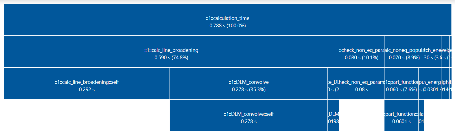
- generate_perf_profile()[source]
Generate a visual/interactive performance profile diagram for the last calculated spectrum, with
tuna.Requires a
profilerkey with in Spectrum.conditions, andtunainstalled.Note
print_perf_profile()is an ascii-version which does not requiretuna.Examples
sf = SpectrumFactory(...)
sf.eq_spectrum(...)
sf.generate_perf_profile()
See typical output in https://github.com/radis/radis/pull/325
Note
You can also profile with
tunadirectly:python -m cProfile -o program.prof your_radis_script.py tuna your_radis_script.py
See also
- misc[source]
Miscellaneous parameters (
MiscParams) params that cannot change the output of calculations (ex: number of CPU, etc.)
- molparam[source]
contains information about molar mass; isotopic abundance.
See
MolParams- Type:
MolParam
- non_eq_spectrum(Tvib=None, Trot=None, Ttrans=None, Telec=None, mole_fraction=None, path_length=None, diluent=None, pressure=None, vib_distribution='boltzmann', rot_distribution='boltzmann', overpopulation=None, name=None) Spectrum[source]
Calculate emission spectrum in non-equilibrium case. Calculates absorption with broadened linestrength and emission with broadened Einstein coefficient.
- Parameters:
Tvib (float) – vibrational temperature [K] can be a tuple of float for the special case of more-than-diatomic molecules (e.g: CO2); only applicable for molecules, not atoms
Trot (float) – rotational temperature [K]; only applicable for molecules, not atoms
Ttrans (float) – translational temperature [K]. If None, translational temperature is taken as rotational temperature (valid at 1 atm for times above ~ 2ns which is the RT characteristic time)
Telec (float) – electronic temperature [K]; only implemented for atoms, not molecules
mole_fraction (float) – database species mole fraction. If None, Factory mole fraction is used.
diluent (str or dictionary) – can be a string of a single diluent or a dictionary containing diluent name as key and its mole_fraction as value
path_length (float or
Quantity) – slab size (cm). IfNone, the default Factorypath_lengthis used.pressure (float or
Quantity) – pressure (bar). IfNone, the default Factorypressureis used.
- Other Parameters:
vib_distribution (
'boltzmann','treanor') – vibrational distributionrot_distribution (
'boltzmann') – rotational distributionoverpopulation (dict, or
None) –add overpopulation factors for given levels:
{level:overpopulation_factor}
name (str) – output Spectrum name (useful in batch)
- Returns:
s –
Returns a
Spectrumobject- Return type:
Examples
from radis import SpectrumFactory
sf = SpectrumFactory(
wavenum_min=2000,
wavenum_max=3000,
molecule="CO",
isotope="1,2,3",
wstep="auto"
)
sf.fetch_databank("hitemp", load_columns='noneq')

s1 = sf.non_eq_spectrum(Tvib=2000, Trot=600, path_length=1, pressure=0.1)
s2 = sf.non_eq_spectrum(Tvib=2000, Trot=600, path_length=1, pressure=0.1)
Multi-vibrational temperature. Below we compare non-LTE spectra of CO2 where all vibrational temperatures are equal, or where the bending and symmetric modes are in equilibrium with rotation
from radis import SpectrumFactory
sf = SpectrumFactory(
wavenum_min=2000,
wavenum_max=3000,
molecule="CO2",
isotope="1,2,3",
)
sf.fetch_databank("hitemp", load_columns='noneq')
# nonequilibrium between bending+symmetric and asymmetric modes :
s1 = sf.non_eq_spectrum(Tvib=(600, 600, 2000), Trot=600, path_length=1, pressure=1)
# all vibrational temperatures are equal :
s2 = sf.non_eq_spectrum(Tvib=(2000, 2000, 2000), Trot=600, path_length=1, pressure=1)
References
See also
- optically_thin_power(Tgas=None, Tvib=None, Trot=None, Ttrans=None, vib_distribution='boltzmann', rot_distribution='boltzmann', mole_fraction=None, path_length=None, unit='mW/cm2/sr')[source]
Calculate total power emitted in equilibrium or non-equilibrium case in the optically thin approximation: it sums all emission integral over the total spectral range.
Warning
this is a fast implementation that doesnt take into account the contribution of lines outside the given spectral range. It is valid for spectral ranges surrounded by no lines, and spectral ranges much broadened than the typical line broadening (~ 1-10 cm-1 in the infrared)
If what you’re looking for is an accurate simulation on a narrow spectral range you better calculate the spectrum (that does take all of that into account) and integrate it with
get_power()- Parameters:
Tgas (float) – equilibrium temperature [K] If doing a non equilibrium case it should be None. Use Ttrans for translational temperature
Tvib (float) – vibrational temperature [K]
Trot (float) – rotational temperature [K]
Ttrans (float) – translational temperature [K]. If None, translational temperature is taken as rotational temperature (valid at 1 atm for times above ~ 2ns which is the RT characteristic time)
mole_fraction (float) – database species mole fraction. If None, Factory mole fraction is used.
path_length (float) – slab size (cm). If None, Factory mole fraction is used.
unit (str) – output unit. Default
'mW/cm2/sr'
- Returns:
float – see
unit=.- Return type:
Returns total power density in mW/cm2/sr (unless different unit is chosen),
See also
- params[source]
Parametersthey may change the output of calculations (ex: threshold, cutoff, broadening methods, etc.)- Type:
Computational parameters
- predict_time()[source]
predict_time(self) uses the input parameters like Spectral Range, Number of lines, wstep, truncation to predict the estimated calculation time for the Spectrum broadening step(bottleneck step) for the current optimization and broadening_method. The formula for predicting time is based on benchmarks performed on various parameters for different optimization, broadening_method and deriving its time complexity.
Benchmarks: https://anandxkumar.github.io/Benchmark_Visualization_GSoC_2021/
Complexity vs Calculation Time Visualizations LBL>Voigt: LINK, DIT>Voigt: LINK, DIT>FFT: LINK
- Returns:
float
- Return type:
Predicted time in seconds.
- print_perf_profile(number_format='{:.3f}', precision=16)[source]
Prints Profiler output dictionary in a structured manner for the last calculated spectrum
Examples
sf.print_perf_profile() # output >> spectrum_calculation 0.189s ████████████████ check_line_databank 0.000s check_non_eq_param 0.042s ███ fetch_energy_5 0.015s █ calc_weight_trans 0.008s reinitialize 0.002s copy_database 0.000s memory_usage_warning 0.002s reset_population 0.000s calc_noneq_population 0.041s ███ part_function 0.035s ██ population 0.006s scaled_non_eq_linestrength 0.005s map_part_func 0.001s corrected_population_se 0.003s calc_emission_integral 0.006s applied_linestrength_cutoff 0.002s calc_lineshift 0.001s calc_hwhm 0.007s generate_wavenumber_arrays 0.001s calc_line_broadening 0.074s ██████ precompute_LDM_lineshapes 0.012s LDM_Initialized_vectors 0.000s LDM_closest_matching_line 0.001s LDM_Distribute_lines 0.001s LDM_convolve 0.060s █████ others 0.001s calc_other_spectral_quan 0.003s generate_spectrum_obj 0.000s others -0.016s- Other Parameters:
precision (int, optional) – total number of blocks. Default 16.
See also
- calc_spectrum(wmin=None, wmax=None, wunit=cm - 1, Tgas=None, Tvib=None, Trot=None, Telec=None, pressure=1.01325, species=None, isotope='all', mole_fraction=1, diluent=None, path_length=1, databank='hitran', medium='air', wstep=0.01, truncation=50, neighbour_lines=0, cutoff=1e-27, parsum_mode='full summation', optimization='simple', chunksize=None, broadening_method='voigt', overpopulation=None, name=None, save_to='', use_cached=True, mode='cpu', export_lines=False, verbose=True, return_factory=False, **kwargs) Spectrum[source]
Calculate a
Spectrum.Can automatically download databases or use manually downloaded local databases, under equilibrium or non-equilibrium, with or without overpopulation, using either CPU or GPU.
It is a wrapper to
SpectrumFactoryclass. For advanced used, please refer to the aforementioned class.- Parameters:
wmin, wmax (float [\(cm^{-1}\)] or
Quantity) –wavelength/wavenumber range. If no units are given, use \(cm^{-1}\)
calc_spectrum(2000, 2300, ... )   # cm-1
calc_spectrum(4000, 4200, wunit='nm', ...)
You can use arbitrary units:
import astropy.units as u
calc_spectrum(2.5*u.um, 3.0*u.um, ...)
wunit (
'nm','cm-1') – unit forwminandwmax. Default is"cm-1".Tgas (float [\(K\)]) – Gas temperature. If non equilibrium, is used for \(T_{translational}\). Default
300KTvib, Trot (float [\(K\)]) – Vibrational and rotational temperatures (for non-LTE calculations). If
None, they are at equilibrium withTgas. Only applicable for molecules, not atoms.Telec (float [\(K\)]) – Electronic temperature (for non-LTE calculations). If
None, it is at equilibrium withTgas. Only implemented for atoms, not molecules.pressure (float [\(bar\)] or
Quantity) –partial pressure of gas in bar. Default
1.01325(1 atm). Use arbitrary units:import astropy.units as u calc_spectrum(..., pressure=20*u.mbar)
species (int, str, list or
None) –- For molecules:
molecule id (HITRAN format) or name. For multiple molecules, use a list. The
'isotope','mole_fraction','databank'and'overpopulation'parameters must then be dictionaries. IfNone, the molecule can be inferred from the database files being loaded. See the list of supported molecules inMOLECULES_LIST_EQUILIBRIUMandMOLECULES_LIST_NONEQUILIBRIUM.- For atoms:
The positive or neutral atomic species. It may be given in spectroscopic notation or any form that can be converted by
to_conventional_name()
Default
None.isotope (int, list, str of the form
'1,2', or'all', or dict) – isotope idFor molecules, this is the isotopologue ID (sorted by relative density: (eg: 1: CO2-626, 2: CO2-636 for CO2) - see [HITRAN-2020] documentation for isotope list for all species.
For atoms, use the isotope number of the isotope (the total number of protons and neutrons in the nucleus) - use 0 to select rows where the isotope is unspecified, in which case the standard atomic weight from the
periodictablemodule is used when mass is required.If
'all', all isotopes in database are used (this may result in larger computation times!).Default
'all'.For multiple molecules, use a dictionary with molecule names as keys
isotope={'CO2':'1,2' , 'CO':'1,2,3' }mole_fraction (float or dict) – database species mole fraction. Default
1.For multiple molecules, use a dictionary with molecule names as keys
mole_fraction={'CO2': 0.8, 'CO':0.2}diluent (str or dictionary) – can be a string of a single diluent or a dictionary containing diluent name as key and its mole_fraction as value For single diluent
diluent = 'CO2'
For multiple diluents
diluent = { 'CO2': 0.6, 'H2O':0.2}
For free electrons, use the symbol ‘e-’. Currently, only H, H2, H2, and e- are supported for atoms - any other diluents have no effect besides diluting the mole fractions of the other constituents.
If left as
None, it defaults to'air'for molecules and atomic hydrogen ‘H’ for atoms.path_length (float [\(cm\)] or
Quantity) –slab size. Default
1cm. Use arbitrary units:import astropy.units as u calc_spectrum(..., path_length=1000*u.km)
databank (str or dict) – can be either: -
'hitran', to fetch the latest HITRAN versionthrough
fetch_hitran()(download full database with [HAPI]) orfetch_astroquery()(download only the required range). To use one mode or the other, usedatabank=('hitran', 'full') # download and cache full database, all isotopes databank=('hitran', 'range') # download and cache required range, required isotope
'hitemp', to fetch the latest HITEMP version throughfetch_hitemp(). Downloads all lines and all isotopes.'exomol', to fetch the latest ExoMol database throughfetch_exomol(). To download a specific database use (more info in fetch_exomol)databank=('exomol', 'EBJT') # 'EBJT' is a specific ExoMol database name
'geisa', to fetch the GEISA 2020 database throughfetch_geisa(). Downloads all lines and all isotopes.the name of a valid database file, in which case the format is inferred. For instance,
'.par'is recognized ashitran/hitempformat. Accepts wildcards'*'to select multiple filesdatabank='PATH/TO/co_*.par'
'kurucz'to fetch the Kurucz linelists for atoms throughfetch_kurucz(). Downloads al lines and all isotopes.'NIST'to fetch the linelists for atoms throughfetch_nist(). Downloads al lines and all isotopes.the name of a spectral database registered in your
~/radis.jsonconfiguration filedatabank='MY_SPECTRAL_DATABASE'
Default
'hitran'. SeeDatabankLoaderfor more information on line databases, andDBFORMATfor your~/radis.jsonfile format.For multiple molecules, use a dictionary with molecule names as keys:
databank='hitran'     # automatic download (or 'hitemp')
databank='PATH/TO/05_HITEMP2019.par'    # path to a file
databank='*CO2*.par' #to get all the files that have CO2 in their names (case insensitive)
databank='HITEMP-2019-CO'   # user-defined database in Configuration file
databank = {'CO2' : 'PATH/TO/05_HITEMP2019.par', 'CO' : 'hitran'}  # for multiple molecules
- Other Parameters:
medium (
'air','vacuum') – propagating medium when giving inputs with'wavenum_min','wavenum_max'. Does not change anything when giving inputs in wavenumber. Default ``’air’``wstep (float (\(cm^{-1}\)) or
'auto') – Resolution of wavenumber grid. Default0.01cm-1. If'auto', it is ensured that there are slightly more or less thanradis.config['GRIDPOINTS_PER_LINEWIDTH_WARN_THRESHOLD']points for each linewidth.Note
wstep = ‘auto’ is optimized for performances while ensuring accuracy, but is still experimental in 0.9.30. Feedback welcome!
truncation (float (\(cm^{-1}\))) – Half-width over which to compute the lineshape, i.e. lines are truncated on each side after
truncation(\(cm^{-1}\)) from the line center. IfNone, use no truncation (lineshapes spread on the full spectral range). Default is50\(cm^{-1}\)Note
Large values (>
50) can induce a performance drop (computation of lineshape typically scale as \(~truncation ^2\) ). The default50was chosen to maintain a good accuracy, and still exhibit the sub-Lorentzian behavior of most lines far (few hundreds \(cm^{-1}\)) from the line center.neighbour_lines (float (\(cm^{-1}\))) – The calculated spectral range is increased (by
neighbour_linescm-1 on each side) to take into account overlaps from out-of-range lines. Default is0\(cm^{-1}\).cutoff (float (~ unit of Linestrength: \(cm^{-1}/(molec.cm^{-2})\))) – discard linestrengths that are lower that this, to reduce calculation times.
1e-27is what is generally used to generate line databases such as CDSD. If0, no cutoff. Default1e-27.parsum_mode (‘full summation’, ‘tabulation’) – how to compute partition functions, at nonequilibrium or when partition function are not already tabulated.
'full summation': sums over all (potentially millions) of rovibrational levels.'tabulation': builds an on-the-fly tabulation of rovibrational levels (500 - 4000x faster and usually accurate within 0.1%). Default'full summation'Note
parsum_mode= ‘tabulation’ is new in 0.9.30, and makes nonequilibrium calculations of small spectra extremely fast. Will become the default after 0.9.31.
optimization (
"simple","min-RMS",None) – If either"simple"or"min-RMS"LDM optimization for lineshape calculation is used:"min-RMS": weights optimized by analytical minimization of the RMS-error (See: [Spectral-Synthesis-Algorithm])"simple": weights equal to their relative position in the grid
If using the LDM optimization, broadening method is automatically set to
'fft'. IfNone, no lineshape interpolation is performed and the lineshape of all lines is calculated. Refer to [Spectral-Synthesis-Algorithm] for more explanation on the LDM method for lineshape interpolation. Default"simple".overpopulation (dict) – dictionary of overpopulation compared to the given vibrational temperature. Default
None. Example:overpopulation = {'CO2' : {'(00`0`0)->(00`0`1)': 2.5, '(00`0`1)->(00`0`2)': 1, '(01`1`0)->(01`1`1)': 1, '(01`1`1)->(01`1`2)': 1 } }export_lines (boolean) – if
True, saves details of all calculated lines in Spectrum. This is necessary to later useline_survey(), but can take some space. DefaultFalse.name (str) – name of the output Spectrum. If
None, a unique ID is generated.save_to (str) – save to a
specfile which contains absorption & emission features, all calculation parameters, and can be opened withload_spec(). File can be reloaded and exported to text formats afterwards, seesavetxt(). If file already exists, replace.use_cached (boolean) – use cached files for line database and energy database. Default
True.verbose (boolean, or int) – If
False, stays quiet. IfTrue, tells what is going on. If>=2, gives more detailed messages (for instance, details of calculation times). DefaultTrue.mode (
'cpu','gpu') – if set to'cpu', computes the spectra purely on the CPU. if set to'gpu', offloads the calculations of lineshape and broadening steps to the GPU making use of parallel computations to speed up the process. GPU computations initiated in this way will use the Vulkan backend; useSpectrumFactoryfor more flexibility. GPU spectra will be returned with exit_gpu=False, so the user should call Spectrum.gpu_exit() when they’re done with GPU computations. Only'cpu'is available for atoms. Default'cpu'.return_factory (bool) – if
True, return theSpectrumFactorythat computes the spectrum. Useful to access computational parameters, the line database, or to start batch-computations from a first spectrum calculation. Ex:s, sf = calc_spectrum(..., return_factory=True, save_memory=False) sf.df1 # see the lines calculated sf.eq_spectrum(...) # new calculation without reloading the database
**kwargs (other inputs forwarded to SpectrumFactory) – For instance:
warnings. SeeSpectrumFactorydocumentation for more details on input.
- Returns:
Spectrum– Output spectrum:SpectrumFactory– if usingreturn_factory=True, the Factory that generated the spectrum is returned. if calculating multiple molecules, a dictionary of factories is returned
References
.. [2] RADIS GPU support: GPU Calculations on RADIS
Examples
Calculate a CO spectrum from the HITRAN database:
from radis import calc_spectrum
s = calc_spectrum(1900, 2300,         # cm-1
                  molecule='CO',
                  isotope='1,2,3',
                  pressure=1.01325,   # bar
                  Tgas=1000,
                  mole_fraction=0.1,
                  databank='hitran',  # or 'hitemp'
                  diluent = "air"     # or {'CO2': 0.1, 'air':0.8}
                  )
s.apply_slit(0.5, 'nm')
s.plot('radiance')
This example uses the
apply_slit()andplot()methods. See alsoline_survey():s.line_survey(overlay='radiance')
Calculate a CO2 spectrum from the CDSD-4000 database:
T_list = [1000.0, 1500.0, 2000.0]
s = calc_spectrum(2200, 2400,   # cm-1
                  molecule='CO2',
                  isotope='1',
                  databank='/path/to/cdsd/databank/in/npy/format/',
                  pressure=0.1,  # bar
                  Tgas=T_list[0],
                  mole_fraction=0.1,
                  mode='gpu',
                  )
s.plot('absorbance', show=False)

for T in T_list[1:]:
    s.recalc_gpu(Tgas=T)
    show = (True if T == T_list[-1] else False)
    s.plot("absorbance", show=show, nfig="same")

s.exit_gpu()
This example uses the
eq_spectrum_gpu()method to calculate the spectrum on the GPU. The databank points to the CDSD-4000 databank that has been pre-processed and stored innumpy.npyformat. Consecutive spectra are calulated using the s.recalc_gpu() method, which uses the GPU to rapidly speed up calculations. Without using consecutive s.recalc_gpu() calls, GPU computations do not provide significant advantage to CPU mode. Refer to the online Examples for more cases, and to the Spectrum page for details on post-processing methods.For more details on how to use the GPU method and process the database, refer to the examples linked above and the documentation on GPU support for RADIS. Other Examples ————–
Calculate and Compare Spectra for Multiple Molecules
Calculate and Compare Spectra for Multiple MoleculesReferences
cite: RADIS is built on the shoulders of many state-of-the-art packages and databases. If using RADIS to compute spectra, make sure you cite all of them, for proper reproducibility and acknowledgement of the work ! See How to cite? and the
cite()method.See also


- spectrum_test(**kwargs)[source]
Generate the first example spectrum with
import radis
s = radis.spectrum_test()
s.plot()
- Other Parameters:
kwargs (sent to
calc_spectrum())