


radis.lbl.base module
Summary
A class to aggregate methods to calculate spectroscopic parameter and populations (and unload factory.py)
BaseFactory is inherited by
BroadenFactory eventually
Routine Listing
PUBLIC METHODS
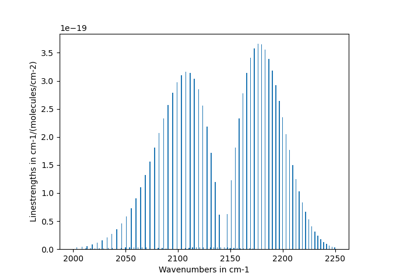
radis.lbl.base.BaseFactory.print_conditions()>>> get all calculation conditionsradis.lbl.base.BaseFactory.get_energy_levels()>>> return energy databaseradis.lbl.base.BaseFactory.plot_linestrength_hist()>>> plot distribution of linestrengths
PRIVATE METHODS - CALCULATE SPECTROSCOPIC PARAMETERS (everything that doesnt depend on populations / temperatures) (computation: work & update with ‘df0’ and called before eq_spectrum() )
radis.lbl.base.BaseFactory._add_EvibErot()radis.lbl.base.BaseFactory._add_EvibErot_CDSD()radis.lbl.base.BaseFactory._add_EvibErot_RADIS_cls1()radis.lbl.base.BaseFactory._add_Evib123Erot_RADIS_cls5()radis.lbl.base.BaseFactory._add_ju()radis.lbl.base.BaseFactory._add_Eu()radis.lbl.base.BaseFactory._calc_noneq_parameters()
PRIVATE METHODS - APPLY ENVIRONMENT PARAMETERS (all functions that depends upon T or P) (calculates populations, linestrength & radiance, lineshift) (computation: work on df1, called by or after eq_spectrum() )
radis.lbl.base.BaseFactory._cutoff_linestrength()
Most methods are written in inherited class with the following inheritance scheme:
DatabankLoader > BaseFactory >
BroadenFactory > BandFactory >
SpectrumFactory
- class BaseFactory[source]
Bases:
DatabankLoader- Qgas(df1, Tgas)[source]
Calculate partition function Qgas at temperature
Tgas, for all lines ofdf1. Returns a single value if all lines have the same Qgas value, or a column if they are different- Parameters:
Tgas (float (K)) – gas temperature
- Returns:
float or dict
- Return type:
Returns Qgas as a dictionary with isotope values as its keys
See also
Qgas_Qref_ratio()
- Qneq(df, Tvib, Trot, vib_distribution, rot_distribution, overpopulation)[source]
Nonequilibrium partition function
- Returns:
column or float
- Return type:
depending if there are many isotopes or one
- Qneq_Qvib_Qrotu_Qrotl(df, Tvib, Trot, vib_distribution, rot_distribution, overpopulation)[source]
Nonequilibrium partition function; with the detail of vibrational partition function and rotational partition functions
- Qref_Qgas_ratio(df1, Tgas, Tref)[source]
Calculate Qref/Qgas at temperature
Tgas,Tref, for all lines ofdf1. Returns a single value if all lines have the same Qref/Qgas ratio, or a column if they are differentSee also
- assert_no_nan(df, column)[source]
Assert there are no nan in the column.
Crash with a nice explanation if one is found
- calc_S0(df)[source]
Calculate the unscaled intensity from the tabulated Einstein coefficient.
- Parameters:
df (DataFrame) – The DataFrame to which the
S0column is to be added- Returns:
None
- Return type:
dfis updated directly with new columnS0
References
\[S_0 = \frac{I_a g' A_{21}}{8 \pi c \nu^2}\]Notes
Currently this value is used in GPU calculations. It is one of the columns that is transferred to the GPU memory. The idea behind S0 is that it is scaled with all variables that do not change during iterations as to minimize calculations.
Units: cm-1/(molecules/cm-2
- NOTE: S0 is not directly related to S(T) used elsewhere!!!
(It may even differ in units!!!)
- calc_einstein_coefficients()[source]
Calculate \(A (= A_{ul})\), \(B_{lu}\), \(B_{ul}\) Einstein coefficients from weighted transition moments squared \(R_s^2\).
- Returns:
None
- Return type:
self.df0is updated directly with new columnsA,Blu,Bul
Note
Einstein A coefficient already in the HITRAN database. In the HITRAN database, the maximum difference betweeen the tabulated and the recalculated values of A was 0.053% for CO2 and 0.099%, see https://github.com/radis/radis/issues/665
References
Einstein induced absorption coefficient (in \(cm^3/J/s^2\))
\[B_{lu}=10^{-36}\cdot\frac{8{\pi}^3}{3h^2} R_s^2 \cdot 10^{-7}\]Einstein induced emission coefficient (in \(cm^3/J/s^2\))
\[B_{ul}=10^{-36}\cdot\frac{8{\pi}^3}{3h^2} \frac{gl}{gu} R_s^2 \cdot 10^{-7}\]Einstein spontaneous emission coefficient (in \(s^{-1}\))
\[A = A_{ul}=10^{-36}\cdot\frac{\frac{64{\pi}^4}{3h} {\nu}^3 gl}{gu} R_s^2\]See (Eqs.(A7), (A8), (A9) in [Rothman-1998])
- calc_emission_integral()[source]
Calculate the emission integral (in \(mW/sr\)) of all lines in DataFrame
df1.\[E_i=\frac{n_u A_{ul}}{4 \pi} \Delta E_{ul}\]Where \(A_{ul}\) (\(s^{-1}\)) is the Einstein coefficient of the corresponding line, \(n_u\) (in \(cm^{-3}/cm^{-3}\) is the fraction of the molecule population in the upper rovibrational state, and \(\Delta E_{ul}\) the transition energy.
Emission Integral is a non usual quantity introduced in RADIS as an equivalent for emission calculations of the Linestrength quantity used in absorption calculations.
The emission integral is later multiplied by the total density \(n_tot\) and the lineshape \(\Phi_i\) to obtain the spectral emission coefficient \(\epsilon_i\) associated to each line.
\[\epsilon_i(\lambda) = E_i \cdot n_{tot} \cdot \Phi_i(\lambda)\]Which are afterwards summed over all N lines to obtain the total emission coefficient :
\[\epsilon(\lambda) = \sum_i^N {\epsilon_i}(\lambda)\]- Returns:
Emission integral
Eiadded indf1- Return type:
None
See also
- calc_lineshift()[source]
Calculate lineshift due to pressure.
- Returns:
None
- Return type:
self.df1is updated directly with new columnshiftwav
References
Shifted line center based on pressure shift coefficient \(lambda_{shift}\) and pressure \(P\).
\[\omega_{shift}=\omega_0+\lambda_{shift} P\]See Eq.(A13) in [Rothman-1998]
- calc_linestrength_eq(Tgas)[source]
Calculate linestrength at temperature Tgas correcting the database linestrength tabulated at temperature \(T_{ref}\).
- Parameters:
Tgas (float (K)) – gas temperature
- Returns:
None
- Return type:
self.df1is updated directly with new columnS
References
\[S(T) = S_0 \frac{Q_{ref}}{Q_{gas}} \operatorname{exp}\left(-E_l \left(\frac{1}{T_{gas}}-\frac{1}{T_{ref}}\right)\right) \frac{1-\operatorname{exp}\left(\frac{-\omega_0}{Tgas}\right)}{1-\operatorname{exp}\left(\frac{-\omega_0}{T_{ref}}\right)}\]See Eq.(A11) in [Rothman-1998]
Notes
Internals:
(some more informations about what this function does)
Starts with df1 which is still a copy of df0 loaded by
load_databank()Updates linestrength in df1. Cutoff criteria is applied afterwards.Examples using
radis.lbl.base.BaseFactory.calc_linestrength_eq¶See also
- calc_linestrength_noneq()[source]
Calculate linestrengths at non-LTE
- Parameters:
Pre-requisite – lower state population
nlhas already been calculated bycalc_populations_noneq()- Returns:
Linestrength
Sadded in self.df- Return type:
None
Notes
Internals:
(some more informations about what this function does)
Starts with df1 which is was a copy of df0 loaded by load_databank(), with non-equilibrium quantities added and populations already calculated. Updates linestrength in df1. Cutoff criteria is applied afterwards.
- calc_populations_eq(Tgas)[source]
Calculate upper state population for all active transitions in equilibrium case (only used in total power calculation)
- Parameters:
Tgas (float (K)) – temperature
- Returns:
nuis stored in self.df1- Return type:
None
Notes
Isotopes: these populations are not corrected for the isotopic abundance, i.e, abundance has to be accounted for if used for emission density calculations (based on Einstein A coefficient), but not for linestrengths (that include the abundance dependency already)
References
Population of upper state follows a Boltzmann distribution:
\[n_u = g_u \frac{\operatorname{exp}\left(\frac{-E_u}{T_{gas}}\right)}{Q_{gas}}\]See also
calc_populations_noneq(),_calc_populations_noneq_multiTvib(),at()
- calc_populations_noneq(Tvib=None, Trot=None, Telec=None, vib_distribution='boltzmann', rot_distribution='boltzmann', overpopulation=None)[source]
Calculate upper and lower state population for all active transitions, as well as all levels (through
at_noneq()for molecules)- Parameters:
Tvib, Trot, Telec (float (K)) – temperatures
vib_distribution (
'boltzmann','treanor') – vibrational level (only applicable for molecules)rot_distribution (
'boltzmann') – rotational level distribution (only applicable for molecules)overpopulation (dict, or
None) – dictionary of overpopulation factors for vibrational levels (only applicable for molecules)
- Returns:
None
- Return type:
nu,nl, (andnu_vib,nl_vibtoo for molecules) are stored in self.df1
Notes
Isotopic abundance:
Note that these populations are not corrected for the isotopic abundance, i.e, abundance has to be accounted for if used for emission density calculations (based on Einstein A coefficient), but not for linestrengths (that include the abundance dependency already)
All populations:
This method calculates populations of emitting and absorbing levels. Populations of all levels (even the one not active on the spectral range considered) are calculated during the Partition function calculation. See:
at_noneq()References
Boltzmann vibrational distributions
\[n_{vib}=\frac{g_{vib}}{Q_{vib}} \operatorname{exp}\left(\frac{-E_{vib}}{T_{vib}}\right)\]or Treanor vibrational distributions
\[n_{vib}=\frac{g_{vib}}{Qvib} \operatorname{exp}\left(-\left(\frac{E_{vib,harm}}{T_{vib}}+\frac{E_{vib,anharm}}{T_{rot}}\right)\right)\]Overpopulation of vibrational levels
\[n_{vib}=\alpha n_{vib}\]Boltzmann rotational distributions
\[n_{rot}=\frac{g_{rot}}{Q_{rot}} \operatorname{exp}\left(\frac{-E_{rot}}{T_{rot}}\right)\]Final rovibrational population of one level
\[n=n_{vib} n_{rot} \frac{Q_{rot} Q_{vib}}{Q}\]See also
calc_populations_eq(),_calc_populations_noneq_multiTvib(),at_noneq()
- calc_weighted_trans_moment()[source]
Calculate weighted transition-moment squared \(R_s^2\) (in
Debye^2)- Returns:
self.df0is updated directly with new columnRs2. R is inDebye^2(1e-36 ergs.cm3)- Return type:
None
References
Weighted transition-moment squared \(R_s^2\) from linestrength \(S_0\) at temperature \(T_{ref}\), derived from Eq.(A5) in [Rothman-1998]
- cond_units0 = {'Tgas': 'K', 'Tref': 'K', 'Trot': 'K', 'Tvib': 'K', 'calculation_time': 's', 'cutoff': 'cm-1/(#.cm-2)', 'neighbour_lines': 'cm-1', 'path_length': 'cm', 'pressure': 'bar', 'truncation': 'cm-1', 'wavelength_max': 'nm', 'wavelength_min': 'nm', 'wavenum_max': 'cm-1', 'wavenum_max_calc': 'cm-1', 'wavenum_min': 'cm-1', 'wavenum_min_calc': 'cm-1', 'wstep': 'cm-1'}[source]
Calculation Conditions units
- df0[source]
initial line database after loading. If for any reason, you want to manipulate the line database manually (for instance, keeping only lines emitting by a particular level), you need to access the
df0attribute ofSpectrumFactory.Warning
never overwrite the
df0attribute, else some metadata may be lost in the process. Only use inplace operations. If reducing the number of lines, add a df0.reset_index()For instance:
from radis import SpectrumFactory
sf = SpectrumFactory(
    wavenum_min= 2150.4,
    wavenum_max=2151.4,
    pressure=1,
    isotope=1)
sf.load_databank('HITRAN-CO-TEST')
sf.df0.drop(sf.df0[sf.df0.vu!=1].index, inplace=True)   # keep lines emitted by v'=1 only
sf.eq_spectrum(Tgas=3000, name='vu=1').plot()
df0contains the lines as they are loaded from the database.df1is generated during the spectrum calculation, after the line database reduction steps, population calculation, and scaling of intensity and broadening parameters with the calculated conditions.See also
df1- Type:
pd.DataFrame
- df1[source]
line database, scaled with populations + linestrength cutoff Never edit manually. See all comments about
df0See also
df0- Type:
pd.DataFrame
- get_energy_levels(molecule, isotope, state='X', conditions=None)[source]
Return energy levels database for given molecule > isotope > state (look up Factory.parsum_calc[molecule][iso][state])
- Parameters:
molecule (str) – molecule name
isotope (int) – isotope identifier
state (str:) – electronic state. Default
'X'(ground-state)conditions (str, or
None) – if not None, add conditions on which energies to retrieve, e.g:>>> 'j==0' or 'v1==0'
Conditions are applied using Dataframe.query() method. In that case,
get_energy_levels()returns a copy. DefaultNone
- Returns:
energies – a view of the energies stored in the Partition Function calculator for isotope iso. If conditions are applied, we get a copy
- Return type:
pandas Dataframe
See also
- get_lines_abundance(df)[source]
Returns the isotopic abundance of each line in
df- Parameters:
df (dataframe)
- Returns:
float or dict
- Return type:
The abundance of all the isotopes in the dataframe
- get_molar_mass(df)[source]
Returns molar mass for all lines of DataFrame
df.- Parameters:
df (pd.DataFrame)
- Return type:
The molar mass of all the isotopes in the dataframe
- get_populations(levels='vib')[source]
For all molecules / isotopes / electronic states, lookup energy levels as calculated in partition function calculators, and (if calculated) populations, and returns as a dictionary.
- Parameters:
levels (
'vib','rovib', list of these, orNone) – what levels to get. Note that'rovib'can yield large Spectrum objects.- Returns:
pops –
Structure:
{molecule: {isotope: {electronic_state: {'vib': pandas Dataframe,    # (copy of) vib levels
                                         'rovib': pandas Dataframe,  # (copy of) rovib levels
                                         'Ia': float    # isotopic abundance
                                         }}}}
- Return type:
dict
See also
- misc[source]
Miscellaneous parameters (
MiscParams) params that cannot change the output of calculations (ex: number of CPU, etc.)
- molparam[source]
contains information about molar mass; isotopic abundance.
See
MolParams- Type:
MolParam
- params[source]
Parametersthey may change the output of calculations (ex: threshold, cutoff, broadening methods, etc.)- Type:
Computational parameters
- plot_hist(dataframe='df0', what='int', axvline=None)[source]
Plot distribution of column
whatindataframeFor instance, help determine a cutoff criteria
plot_hist("df1", "int")
- Parameters:
dataframe (‘df0’, ‘df1’) – which dataframe to plot (df0 is the loaded one, df1 the scaled one)
what (str) – which feature to plot. Default
'S'(scaled linestrength). Could also be'int'(reference linestrength intensity),'A'(Einstein coefficient)axvline (float) – if not
None, plot a vertical line at this position.
- plot_linestrength_hist(cutoff=None)[source]
Plot linestrength distribution (to help determine a cutoff criteria)
Examples
s, sf = calc_spectrum(..., return_factory=True)
sf.plot_linestrength_hist()
- plot_populations(what='vib', isotope=None, nfig=None)[source]
Plot populations currently calculated in factory.
Plot populations of all levels that participate in the partition function. Output is different from the Spectrum
plot_populations()method, where only the levels that directly contribute to the spectrum are shownNote: only valid after calculating non_eq spectrum as it uses the partition function calculator object
- Parameters:
what (‘vib’, ‘rovib’) – what levels to plot
isotope (int, or
None) – which isotope to plot. IfNoneand if there are more than one isotope, raises an error.
- Other Parameters:
nfig (int, or str) – on which Figure to plot. Default
None
- print_conditions(prepend=None)[source]
Prints all physical / computational parameters. These are also stored in each result Spectrum.
- Parameters:
prepend (str) – just to text to display before printing conditions
- save_memory[source]
if True, tries to save RAM memory (but may take a little for time, saving stuff to files instead of RAM for instance)
- Type:
bool
- units0 = {'abscoeff': 'cm-1', 'abscoeff_continuum': 'cm-1', 'absorbance': '', 'emisscoeff': 'mW/cm3/sr/cm-1', 'emisscoeff_continuum': 'mW/cm3/sr/cm-1', 'emissivity_noslit': '', 'radiance_noslit': 'mW/cm2/sr/cm-1', 'transmittance_noslit': '', 'waverange': 'cm-1'}[source]
Default output units … may be changed at the initialisation of the SpectrumFactory, for instance … if user gives wavelength units we want to return radiance in … “mW/cm2/sr/nm” units for consistency
- get_wavenumber_range(wmin=None, wmax=None, wunit=cm - 1, wavenum_min=None, wavenum_max=None, wavelength_min=None, wavelength_max=None, medium='air', return_input_wunit=False)[source]
Returns wavenumber based on whatever input was given: either ν_min, ν_max directly, or λ_min, λ_max in the given propagation
medium.- Parameters:
medium (
'air','vacuum') – propagation mediumwmin, wmax (float, or
QuantityorNone) – hybrid parameters that can serve as both wavenumbers or wavelength depending on the unit accompanying them. If unitless, wunit is assumed as the accompanying unit.wunit (string) – The unit accompanying wmin and wmax. Cannot be passed without passing values for wmin and wmax. Default: cm-1
wavenum_min, wavenum_max (float, or
QuantityorNone) – wavenumberswavelength_min, wavelength_max (float, or
QuantityorNone) – wavelengths in givenmedium
- Returns:
wavenum_min, wavenum_max (float) – wavenumbers
input_wunit (‘nm’, ‘nm_vac’, ‘cm-1’) – in which wavespace was the input given before conversion (used to keep default plot/get consistent with input units)
- linestrength_from_Einstein(A, gu, El, Ia, nu, Q, T)[source]
Calculate linestrength at temperature
Tfrom Einstein coefficients.- Parameters:
A (float, s-1) – Einstein emission coefficients
gu (int) – upper state degeneracy
El (float, cm-1) – lower state energy
Ia (float) – isotope abundance
nu (cm-1) – transition wavenumber
Q (float) – partition function at temperature
TT (float) – temperature
- Returns:
S – linestrength at temperature
T.- Return type:
float
References
\[S(T) =\frac{1}{8\pi c_{CGS} {\nu}^2} A \frac{I_a g_u \operatorname{exp}\left(\frac{-c_2 E_l}{T}\right)}{Q(T)} \left(1-\operatorname{exp}\left(\frac{-c_2 \nu}{T}\right)\right)\]Combine Eq.(A.5), (A.9) in [Rothman-1998]
See also