


Line-by-line module
This is the core of RADIS: it calculates the spectral densities for a homogeneous
slab of gas, and returns a Spectrum object.
Calculations are performed within the SpectrumFactory class.
calc_spectrum() is a high-level wrapper to
SpectrumFactory for most simple cases.


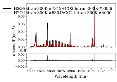
Calculate and Compare Spectra for Multiple Molecules

Line databases
List of supported line databases formats: KNOWN_DBFORMAT.
The databases are stored in a hidden folder ~/.radisdb on the user’s computer.
The informations regarding each database are stored in the configuration file ~/radis.json, see the Configuration file section.
HITRAN / HITEMP
HITRAN is designed for atmospheric applications. It is the most widely used line database. The HITRAN group also supports the HITEMP database, which is designed for high-temperature applications. The files of the HITEMP database are formatted in the same way as HITRAN files but are much larger.
By default, RADIS automatically fetch HITRAN/HITEMP lines using the Astroquery
module. This is done by specifying databank=='hitran' or databank=='hitemp'.
- See the following example for calc_spectrum()
from radis import calc_spectrum
calc_spectrum(
    wavenum_min=2500 / u.cm,
    wavenum_max=4500 / u.cm,
    molecule="OH",
    Tgas=600,
    databank="hitemp",  # test by fetching directly
    verbose=False,
)
If you just want to parse the HITEMP files, use
fetch_hitemp(). You can also refer tofetch_astroquery()for more information.from radis.io.hitemp import fetch_hitemp fetch_hitemp("NO")
You can also download the HITRAN/HITEMP databases files locally, but you will have to properly refer to your database in ~/radis.json.
Note
RADIS has parsers to read line databases in Pandas dataframes.
This can be useful if you want to edit the database.
see hit2df()
There are also functions to get HITRAN molecule ids, and vice-versa:
get_molecule(), get_molecule_identifier()
GEISA
The GEISA database is designed for atmospheric applications. Using GEISA in RADIS is similar to the HITRAN database, simply specify databank=='geisa'.
CDSD-4000
RADIS can read files from the CDSD-4000 database, however files have to be downloaded manually.
CDSD-4000 files can be downloaded from ftp://ftp.iao.ru/pub/. Expect ~50 Gb for all CO2. Cite with [CDSD-4000].
Tabulated partition functions are available in the
partition_functions.txtfile on the [CDSD-4000] FTP : ftp://ftp.iao.ru/pub/CDSD-4000/ . They can be loaded and interpolated withPartFuncCO2_CDSDtab. This can be done automatically providingparfuncfmt: cdsdandparfunc = PATH/TO/cdsd_partition_functions.txtis given in the~/radis.jsonconfiguration file (see the Configuration file).
The ~/radis.json is used to properly handle the line databases
on the User environment. See the Configuration file section, as well as
the radis.misc.config module and the getDatabankList()
function for more information.
Note
See cdsd2df() for the conversion to a Pandas DataFrame.
Calculating spectra
Calculate one molecule spectrum
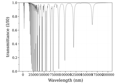
In the following example, we calculate a CO spectrum at equilibrium from the latest HITRAN database, and plot the transmittance:
s = calc_spectrum(
                wavenum_min=1900,
                wavenum_max=2300,
                Tgas=700,
                path_length=0.1,
                molecule='CO',
                mole_fraction=0.5,
                isotope=1,
    wstep=0.01,
    databank='hitran'   # or 'hitemp'
                )
s.plot('transmittance_noslit')
Calculate multiple molecules spectrum
RADIS can also calculate the spectra of multiple molecules. In the following example, we add the contribution of CO2 and plot the transmittance:
s = calc_spectrum(
        wavenum_min=1900,
        wavenum_max=2300,
        Tgas=700,
        path_length=0.1,
        mole_fraction={'CO2':0.5, 'CO':0.5},
        wstep=0.01,
  isotope=1,
        )
s.plot('transmittance_noslit')
Note that you can indicate the considered molecules either as a list
in the molecule parameter, or in isotope or mole_fraction. The
following commands give the same result:
# Give molecule:
s = calc_spectrum(
        wavelength_min=4165,
        wavelength_max=5000,
        Tgas=1000,
        path_length=0.1,
        molecule=["CO2", "CO"],
        mole_fraction=1,
        isotope={"CO2": "1,2", "CO": "1,2,3"},
        wstep=0.01,
        verbose=verbose,
  )


# Give isotope only
s = calc_spectrum(
    wavelength_min=4165,
    wavelength_max=5000,
    Tgas=1000,
    path_length=0.1,
    isotope={"CO2": "1,2", "CO": "1,2,3"},
    verbose=verbose,
)

# Give mole fractions only
s = calc_spectrum(
    wavelength_min=4165,
    wavelength_max=5000,
    Tgas=1000,
    path_length=0.1,
    mole_fraction={"CO2": 0.2, "CO": 0.8},
    isotope="1,2",
    verbose=verbose,
)
Be careful to be consistent and not to give partial or contradictory inputs.
# Contradictory input:
s = calc_spectrum(
         wavelength_min=4165,
         wavelength_max=5000,
         Tgas=1000,
         path_length=0.1,
         molecule=["CO2"],  # contradictory
         mole_fraction=1,
         isotope={"CO2": "1,2", "CO": "1,2,3"},
         verbose=verbose,
     )

 # Partial input:
 s = calc_spectrum(
         wavelength_min=4165,
         wavelength_max=5000,
         Tgas=1000,
         path_length=0.1,
         molecule=["CO2", "CO"],  # contradictory
         mole_fraction=1,
         isotope={"CO2": "1,2"},  # unclear for CO
         verbose=verbose,
     )
Equilibrium Conditions
By default RADIS calculates spectra at thermal equilibrium (one temperature).
The calc_spectrum() function requires a
given mole fraction, which may be different from chemical equilibrium.
You can also compute the chemical equilibrium composition in
other codes like [CANTERA], and feed the output to
RADIS calc_spectrum(). The
get_eq_mole_fraction() function
provides an interface to [CANTERA] directly from RADIS
from radis import calc_spectrum, get_eq_mole_fraction

# calculate gas composition of a 50% CO2, 50% H2O mixture at 1600 K:
gas = get_eq_mole_fraction('CO2:0.5, H2O:0.5', 1600, # K
                                     1e5  # Pa
                           )
# calculate the contribution of H2O to the spectrum:
calc_spectrum(...,
              mole_fraction=gas['H2O']
              )
Nonequilibrium Calculations
Non-LTE calculations (multiple temperatures) require to know the vibrational and rotational energies of each level in order to calculate the nonequilibrium populations.
You can either let RADIS calculate rovibrational energies with its built-in spectroscopic constants, or supply an energy level database. In the latter case, you need to edit the Configuration file .
Calculating spectrum using GPU
RADIS also supports CUDA-native parallel computation, specifically
for lineshape calculation and broadening. To use these GPU-accelerated methods to compute the spectra, use either calc_spectrum()
function with parameter mode set to gpu, or eq_spectrum_gpu(). In order to use these methods,
ensure that your system has an Nvidia GPU with compute capability of at least 3.0 and CUDA Toolkit 8.0 or above. Refer to
GPU Spectrum Calculation on RADIS to see how to setup your system to run GPU accelerated spectrum
calculation methods, examples and performance tests.
Currently, GPU-powered spectra calculations are supported only at thermal equilibrium
and therefore, the method to calculate the spectra has been named eq_spectrum_gpu().
In order to use this method to calculate the spectra, follow the same steps as in the
case of a normal equilibrium spectra, and if using calc_spectrum()
function set the parameter mode to gpu, or use eq_spectrum_gpu()
One could compute the spectra with the assistance of GPU using the following code as well
s = calc_spectrum(
            wavenum_min=1900,
            wavenum_max=2300,
            Tgas=700,
            path_length=0.1,
            mole_fraction=0.01,
            isotope=1,
            mode='gpu'
            )
Refer to GPU Spectrum Calculation on RADIS for more details.
Under the hood
Flow Chart
RADIS can calculate populations of emitting/absorbing levels by scaling tabulated data (equilibrium) or from the rovibrational energies (nonequilibrium), get the emission and absorption coefficients from Line Databases, calculate the line broadening using various strategies to improve Performances, and produce a Spectrum object. These steps can be summarized in the flow chart below:

The detail of the functions that perform each step of the RADIS calculation flow chart is given in Architecture.
The Spectrum Factory
Most RADIS calculations can be done using the calc_spectrum() function.
Advanced examples require to use the SpectrumFactory
class, which is the core of RADIS line-by-line calculations.
calc_spectrum() is a wrapper to SpectrumFactory
for the simple cases.
The SpectrumFactory allows you to :
calculate multiple spectra (batch processing) with a same line database
edit the line database manually
have access to intermediary calculation variables
connect to a database of precomputed spectra on your computer
To use the SpectrumFactory, first
load your own line database with load_databank(),
and then calculate several spectra in batch using
eq_spectrum() and
non_eq_spectrum(),
and units
import astropy.units as u
from radis import SpectrumFactory
sf = SpectrumFactory(wavelength_min=4165 * u.nm,
                     wavelength_max=4200 * u.nm,
                     path_length=0.1 * u.m,
                     pressure=20 * u.mbar,
                     molecule='CO2',
                     wstep = 0.01,
                     isotope='1,2',
                     cutoff=1e-25,              # cm/molecule
                     broadening_max_width=10,   # cm-1
                     )
sf.load_databank('HITRAN-CO2-TEST', load_columns='noneq')        # this database must be defined in ~/radis.json
s1 = sf.eq_spectrum(Tgas=300 * u.K)
s2 = sf.eq_spectrum(Tgas=2000 * u.K)
s3 = sf.non_eq_spectrum(Tvib=2000 * u.K, Trot=300 * u.K)
Note that for non-LTE calculations, specific columns must be loaded. This is done by using the
load_columns='noneq' parameter. See load_databank()
for more information.
Configuration file
The ~/radis.json configuration file is used to initialize your radis.config.
It will :
store the list and attributes of the Line databases available on your computer.
change global user preferences, such as plotting styles and libraries, or warnings thresholds, or default algorithms.
The list of all available parameters is given in the default_radis.json
file. Any key added to your ~/radis.json will override the value of
default_radis.json.
Note
You can also update config parameters at runtime by setting:
import radis
radis.config["SOME_KEY"] = "SOME_VALUE"
Although it is recommended to simply edit your ~/radis.json file.
Databases downloaded from ‘hitran’, ‘hitemp’ and ‘exomol’ with calc_spectrum()
or fetch_databank() are automatically
registered in the ~/radis.json configuration file. The default download path
is ~/.radisdb. You can change this at runtime by setting the radis.config["DEFAULT_DOWNLOAD_PATH"]
key, or (recommended) by adding a DEFAULT_DOWNLOAD_PATH key in your ~/radis.json
configuration file.
The configuration file will help to:
handle local line databases that contains multiple files
use custom tabulated partition functions for equilibrium calculations
use custom, precomputed energy levels for nonequilibrium calculations
Note
It is also possible to work with local line databases without a configuration file,
either by giving a file to the databank=... parameter of calc_spectrum() ,
or by giving to load_databank() the line database path,
format, and partition function format directly.
However, this is not recommended and should only be used if for some reason you cannot create a configuration file.
A ~/radis.json is user-dependant, and machine-dependant. It contains a list of database, each of which
is specific to a given molecule. Typical expected format of a ~/radis.json entry:
{
  "database": {                                     # database key: all databanks information are stored in this key
      "MY-HITEMP-CO2": {                            # your databank name: use this in calc_spectrum()
                                                    # or SpectrumFactory.load_databank()
        "path": [                                   # no "", multipath allowed
            "D:\\Databases\\HITEMP-CO2\\hitemp_07",
            "D:\\Databases\\HITEMP-CO2\\hitemp_08",
            "D:\\Databases\\HITEMP-CO2\\hitemp_09"
        ],
        "format": "hitran",                         # 'hitran' (HITRAN/HITEMP), 'cdsd-hitemp', 'cdsd-4000'
                                                    # databank text file format. More info in
                                                    # SpectrumFactory.load_databank function.
      }
  }
}
Following is an example where the path variable uses a wildcard * to find all the files that have hitemp_* in their names:
{
  "database": {                                     # database key: all databanks information are stored in this key
      "MY-HITEMP-CO2": {                            # your databank name: use this in calc_spectrum()
                                                    # or SpectrumFactory.load_databank()
        "path": "D:\\Databases\\HITEMP-CO2\\hitemp_*",   # To load all hitemp files directly
        "format": "hitran",                         # 'hitran' (HITRAN/HITEMP), 'cdsd-hitemp', 'cdsd-4000'
                                                    # databank text file format. More info in
                                                    # SpectrumFactory.load_databank function.
      }
  }
}
In the former example, for equilibrium calculations, RADIS uses [HAPI] to retrieve partition functions tabulated with TIPS-2017. It is also possible to use your own partition functions, for instance:
{
  "database": {                                       # database key: all databanks information are stored in this key
      "MY-HITEMP-CO2": {                              # your databank name: use this in calc_spectrum()
                                                      # or SpectrumFactory.load_databank()
        "path": [                                     # no "", multipath allowed
            "D:\\Databases\\HITEMP-CO2\\hitemp_07",
            "D:\\Databases\\HITEMP-CO2\\hitemp_08",
            "D:\\Databases\\HITEMP-CO2\\hitemp_09"
        ],
        "format": "hitran",                           # 'hitran' (HITRAN/HITEMP), 'cdsd-hitemp', 'cdsd-4000'
                                                      # databank text file format. More info in
                                                      # SpectrumFactory.load_databank function.
        "parfunc": "PATH/TO/cdsd_partition_functions.txt"
                                                      # path to tabulated partition function to use.
                                                      # If not given, then the hapi.py embedded in RADIS
                                                      # is used (check version)
      }
  }
}
By default, for nonequilibrium calculations, RADIS built-in spectroscopic constants are used to calculate the energy levels for CO2. It is also possible to use your own Energy level database. For instance:
{
  "database": {                                        # database key: all databanks information are stored in this key
      "MY-HITEMP-CO2": {                               # your databank name: use this in calc_spectrum()
                                                       # or SpectrumFactory.load_databank()
        "path": [                                      # no "", multipath allowed
            "D:\\Databases\\HITEMP-CO2\\hitemp_07",
            "D:\\Databases\\HITEMP-CO2\\hitemp_08",
            "D:\\Databases\\HITEMP-CO2\\hitemp_09"
        ],
        "format": "hitran",                             # 'hitran' (HITRAN/HITEMP), 'cdsd-hitemp', 'cdsd-4000'
                                                        # databank text file format. More info in
                                                        # SpectrumFactory.load_databank function.
                                                        # is used (check version)
        "levels_iso1": "D:\\PATH_TO\\energies_of_626_isotope.levels",
        "levels_iso2": "D:\\PATH_TO\\energies_of_636_isotope.levels",
        "levelsfmt": "cdsd",                            # 'cdsd', etc.
                                                        # how to read the previous file. Default None.
        "levelszpe": "2531.828"                         # zero-point-energy (cm-1): offset for all level
                                                        # energies. Default 0 (if not given)
      }
  }
}
The full description of a json entry is given in DBFORMAT:
pathcorresponds to Line databases (here: downloaded from [HITEMP-2010]) and thelevels_isoare user generated Energy databases (here: calculated from the [CDSD-4000] Hamiltonian on non-distributed code, which takes into account non diagonal coupling terms).formatis the databank text file format. It can be one of'hitran'(for HITRAN / HITEMP 2010),'cdsd-hitemp'and'cdsd-4000'for the different CDSD versions (for CO2 only). See full list inKNOWN_DBFORMAT.parfuncis the path to the tabulated partition function to use in in equilibrium calculations (eq_spectrum()). If not given, then thehapiembedded in RADIS is used (check version)levels_iso#are the path to the energy levels to use for each isotope, which are needed for nonequilibrium calculations (non_eq_spectrum()).levelsfmtis the energy levels database format. Typically,'radis', and various implementation of [CDSD-4000] nonequilibrium partitioning of vibrational and rotational energy:'cdsd-pc','cdsd-pcN','cdsd-hamil'. See full list inKNOWN_LVLFORMAT
How to create the configuration file?
A default ~/radis.json configuration file can be generated with setup_test_line_databases(), which
creates two test databases from fragments of [HITRAN-2020] line databases:
from radis.test.utils import setup_test_line_databases
setup_test_line_databases()
which will create a ~/radis.json file with the following content
{
  "database": {
      "HITRAN-CO2-TEST": {
        "info": "HITRAN 2016 database, CO2, 1 main isotope (CO2-626), bandhead: 2380-2398 cm-1 (4165-4200 nm)",
        "path": "PATH_TO\\radis\\radis\\test\\files\\hitran_co2_626_bandhead_4165_4200nm.par",
        "format": "hitran",
        "levelsfmt": "radis"
      },
      "HITRAN-CO-TEST": {
        "info": "HITRAN 2016 database, CO, 3 main isotopes (CO-26, 36, 28), 2000-2300 cm-1",
        "path": "PATH_TO\\radis\\radis\\test\\files\\hitran_co_3iso_2000_2300cm.par",
        "format": "hitran",
        "levelsfmt": "radis"
      },
      "HITEMP-CO2-TEST": {
        "info": "HITEMP-2010, CO2, 3 main isotope (CO2-626, 636, 628), 2283.7-2285.1 cm-1",
        "path": "PATH_TO\\radis\\radis\\test\\files\\cdsd_hitemp_09_fragment.txt",
        "format": "cdsd-hitemp",
        "levelsfmt": "radis"
      }
  }
}
If you configuration file exists already, the test databases will simply be appended.
Advanced
Calculation Flow Chart
Refer to Architecture for an overview of how equilibrium and nonequilibrium calculations are conducted.
Use Custom Spectroscopic constants
Spectroscopic constants are a property of the RADIS ElectronicState
class. All molecules are stored in the Molecules dictionary.
You need to update this dictionary before running your calculation in order to use your
own spectroscopic constants.
An example of how to use your own spectroscopic constants:
from radis import calc_spectrum
from radis.db.molecules import Molecules, ElectronicState

Molecules['CO2'][1]['X'] = ElectronicState('CO2', isotope=1, state='X', term_symbol='1Σu+',
                            spectroscopic_constants='my_constants.json',  # <<< YOUR FILE HERE
                            spectroscopic_constants_type='dunham',
                            Ediss=44600,
                            )
s = calc_spectrum(...)

Vibrational bands
To calculate vibrational bands of a given spectrum separately (vibrational-state-specific calculations), use the
eq_bands() and non_eq_bands()
methods. See the test_plot_all_CO2_bandheads() example in
radis/test/lbl/test_bands.py for more information.
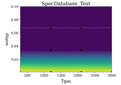
Connect to a Spectrum Database
In RADIS, the same code can be used to retrieve precomputed spectra if they exist, or calculate them and store them if they don’t. See Precompute Spectra and the following example:
Example #7: Database fitting using SpecDatabase.fit_spectrum
Performance
RADIS is very optimized, making use of C-compiled libraries (NumPy, Numba) for computationally intensive steps, and data analysis libraries (Pandas) to handle lines databases efficiently. Additionally, different strategies and parameters are used to improve performances further:
Line Database Reduction Strategies
By default:
linestrength cutoff : lines with low linestrength are discarded after the new populations are calculated. Parameter:
cutoff(see the default value in the arguments ofeq_spectrum())
Additional strategies (deactivated by default):
weak lines (pseudo-continuum): lines which are close to a much stronger line are called weak lines. They are added to a pseudo-continuum and their lineshape is calculated with a simple rectangular approximation. This feature will be deprecated in the future. See the default value in the arguments of
pseudo_continuum_threshold(see arguments ofeq_spectrum())
Lineshape optimizations
Lineshape convolution is usually the performance bottleneck in any line-by-line code.
Two approaches can be used:
improve the convolution efficiency. This involves using an efficient convolution algorithm, using a reduced convolution kernel, analytical approximations, or multiple spectral grid.
reduce the number of convolutions (for a given number of lines): this is done using the LDM strategy.
RADIS implements the two approaches as well as various strategies and parameters to calculate the lineshapes efficiently.
LDM : lines are projected on a Lineshape database to reduce the number of calculated lineshapes from millions to a few dozens. With this optimization strategy, the lineshape convolution becomes almost instantaneous and all the other strategies are rendered useless. Projection of all lines on the lineshape database becomes the performance bottleneck. Parameters:
ldm_res_L,ldm_res_G. (this is the default strategy implemented in RADIS). Learn more in [Spectral-Synthesis-Algorithm]broadening width : lineshapes are calculated on a reduced spectral range because the Voigt computation times scale linearly with that parameter. (Gaussian x Lorentzian calculation times scale as a square with that parameter.) Parameters:
broadening_max_widthVoigt approximation : Voigt is calculated with an analytical approximation. Parameter :
broadening_max_widthand default values in the arguments ofeq_spectrum(). Seevoigt_lineshape().Fortran precompiled : previous Voigt analytical approximation is precompiled in Fortran to improve performance times. This is always the case and cannot be changed on the user side at the moment. See the source code of
voigt_lineshape().Multiple spectral grids : many LBL codes use different spectral grids to calculate the lineshape wings with a lower resolution. This strategy is not implemented in RADIS.
Recommandations for speeding up spectra computations
If performance is an issue (for instance when calculating polyatomic spectra on large spectral ranges), you
may want to tweak the computation parameters in calc_spectrum() and
SpectrumFactory. In particular, the parameters that have the highest
impact on the calculation performances are:
The
broadening_max_width, which defines the spectral range over which the broadening is calculated.The linestrength
cutoff, which defines which low intensity lines should be discarded. Seeplot_linestrength_hist()to choose a correct cutoff.The
pseudo_continuum_thresholddefines a threshold to integrate weak lines into a continuum. This solution will be deprecated in the future.
Check the [RADIS-2018] article for a quantitative assessment of the influence of the different parameters.
See the test_abscoeff_continuum() case in radis/test/lbl/test_broadening.py
for an example, which can be run with (you will need the CDSD-HITEMP database installed)
pytest radis/test/lbl/test_broadening.py -m "test_abscoeff_continuum"
Choose the right wavenumber grid
wstep determines the wavenumber grid’s resolution. Smaller the value, higher the resolution and
vice-versa. By default radis uses wstep=0.01. You can manually set the wstep value
in calc_spectrum() and SpectrumFactory.
To get more accurate result you can further reduce the value, and to increase the performance you can increase the value.
Based on wstep, it will determine the number of gridpoints per linewidth.
To make sure that there are enough gridpoints, Radis will raise an Accuracy Warning _check_accuracy()
if number of gridpoints are less than GRIDPOINTS_PER_LINEWIDTH_WARN_THRESHOLD and raises an Accuracy Error
if number of gridpoints are less than GRIDPOINTS_PER_LINEWIDTH_ERROR_THRESHOLD.
From 0.9.30 a new mode wstep='auto' has been added which directly computes the optimum value of wstep
ensuring both performance and accuracy. It is ensured that there are slightly more or less than GRIDPOINTS_PER_LINEWIDTH_WARN_THRESHOLD
points for each linewidth.
Note
wstep = ‘auto’ is optimized for performances while ensuring accuracy, but is still experimental in 0.9.30. Feedback welcome!
Sparse wavenumber grid
To compute large band spectra with a small number of lines, RADIS includes
a sparse wavenumber implementation of the DIT algorithm, which is
activated based on a scarcity criterion (Nlines/Ngrid_points > 1).
The sparse version can be forced to be activated or deactivated. This behavior
is done by setting the SPARSE_WAVENUMBER key of the radis.config
dictionary, or of the ~/radis.json user file.
See the HITRAN full-range example for an example.
Database loading
Line database can be a performance bottleneck, especially for large polyatomic molecules in the [HITEMP-2010]
or [CDSD-4000] databases.
Line database files are automatically cached by RADIS under a .h5 format after they are loaded the first time.
If you want to deactivate this behaviour, use use_cached=False in calc_spectrum(),
or db_use_cached=False, lvl_use_cached=False in SpectrumFactory.
You can also use init_databank() instead of the default
load_databank(). The former will save the line database parameter,
and only load them if needed. This is useful if used in conjunction with
init_database(), which will retrieve precomputed spectra from
a database if they exist.
Manipulate the database
If for any reason, you want to manipulate the line database manually (for instance, keeping only lines emitting
by a particular level), you need to access the df0 attribute of
SpectrumFactory.
Warning
never overwrite the df0 attribute, else some metadata may be lost in the process. Only use inplace operations.
For instance:
sf = SpectrumFactory(
    wavenum_min= 2150.4,
    wavenum_max=2151.4,
    pressure=1,
    isotope=1)
sf.load_databank('HITRAN-CO-TEST')
sf.df0.drop(sf.df0[sf.df0.vu!=1].index, inplace=True)   # keep lines emitted by v'=1 only
sf.eq_spectrum(Tgas=3000, name='vu=1').plot()
df0 contains the lines as they are loaded from the database.
df1 is generated during the spectrum calculation, after the
line database reduction steps, population calculation, and scaling of intensity and broadening parameters
with the calculated conditions.
Tabulated Partition Functions
At nonequilibrium, calculating partition functions by full summation
of all rovibrational levels can become costly. Radis offers to tabulate
them just-in-time, using the parsum_mode='tabulation' of
calc_spectrum() or SpectrumFactory.
See parsum_mode.
Profiler
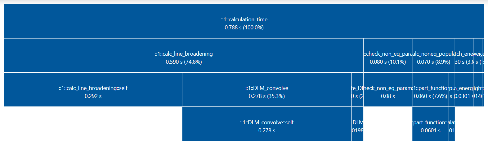
You may want to track where the calculation is taking some time.
You can set verbose=1 or higher to print the time spent on the different
calculation steps at runtime. Example with verbose=3:
s = calc_spectrum(1900, 2300,         # cm-1
                  molecule='CO',
                  isotope='1,2,3',
                  pressure=1.01325,   # bar
                  Tvib=1000,          # K
                  Trot=300,           # K
                  mole_fraction=0.1,
                  verbose=3,
                  )
Performance profiles are kept in the output spectrum Spectrum.profiler dictionary.
You can also use the print_perf_profile()
method in the SpectrumFactory object or the print_perf_profile()
method in the Spectrum object to print them in the console :
For the above example:
s.print_perf_profile()
# Output:
    spectrum_calculation      0.189s ████████████████
        check_line_databank              0.000s
        check_non_eq_param               0.042s ███
        fetch_energy_5                   0.015s █
        calc_weight_trans                0.008s
        reinitialize                     0.002s
            copy_database                    0.000s
            memory_usage_warning             0.002s
            reset_population                 0.000s
        calc_noneq_population            0.041s ███
            part_function                    0.035s ██
            population                       0.006s
        scaled_non_eq_linestrength       0.005s
            map_part_func                    0.001s
            corrected_population_se          0.003s
        calc_emission_integral           0.006s
        applied_linestrength_cutoff      0.002s
        calc_lineshift                   0.001s
        calc_hwhm                        0.007s
        generate_wavenumber_arrays       0.001s
        calc_line_broadening             0.074s ██████
            precompute_LDM_lineshapes        0.012s
            LDM_Initialized_vectors          0.000s
            LDM_closest_matching_line        0.001s
            LDM_Distribute_lines             0.001s
            LDM_convolve                     0.060s █████
            others                           0.001s
        calc_other_spectral_quan         0.003s
        generate_spectrum_obj            0.000s
        others                           -0.016s
Finally, you can also use the SpectrumFactory generate_perf_profile()
Spectrum generate_perf_profile()
methods to generate an interactive profiler in the browser.
Predict Time
predict_time() function uses the input parameters like Spectral Range, Number of lines, wstep,
truncation to predict the estimated calculation time for the Spectrum
broadening step(bottleneck step) for the current optimization and broadening_method. The formula
for predicting time is based on benchmarks performed on various parameters for different optimization,
broadening_method and deriving its time complexity.
The following Benchmarks were used to derive the time complexity:
Complexity vs Calculation Time Visualizations for different optimizations and broadening_method:
Precompute Spectra
See init_database(), which is the direct integration
of SpecDatabase in a SpectrumFactory