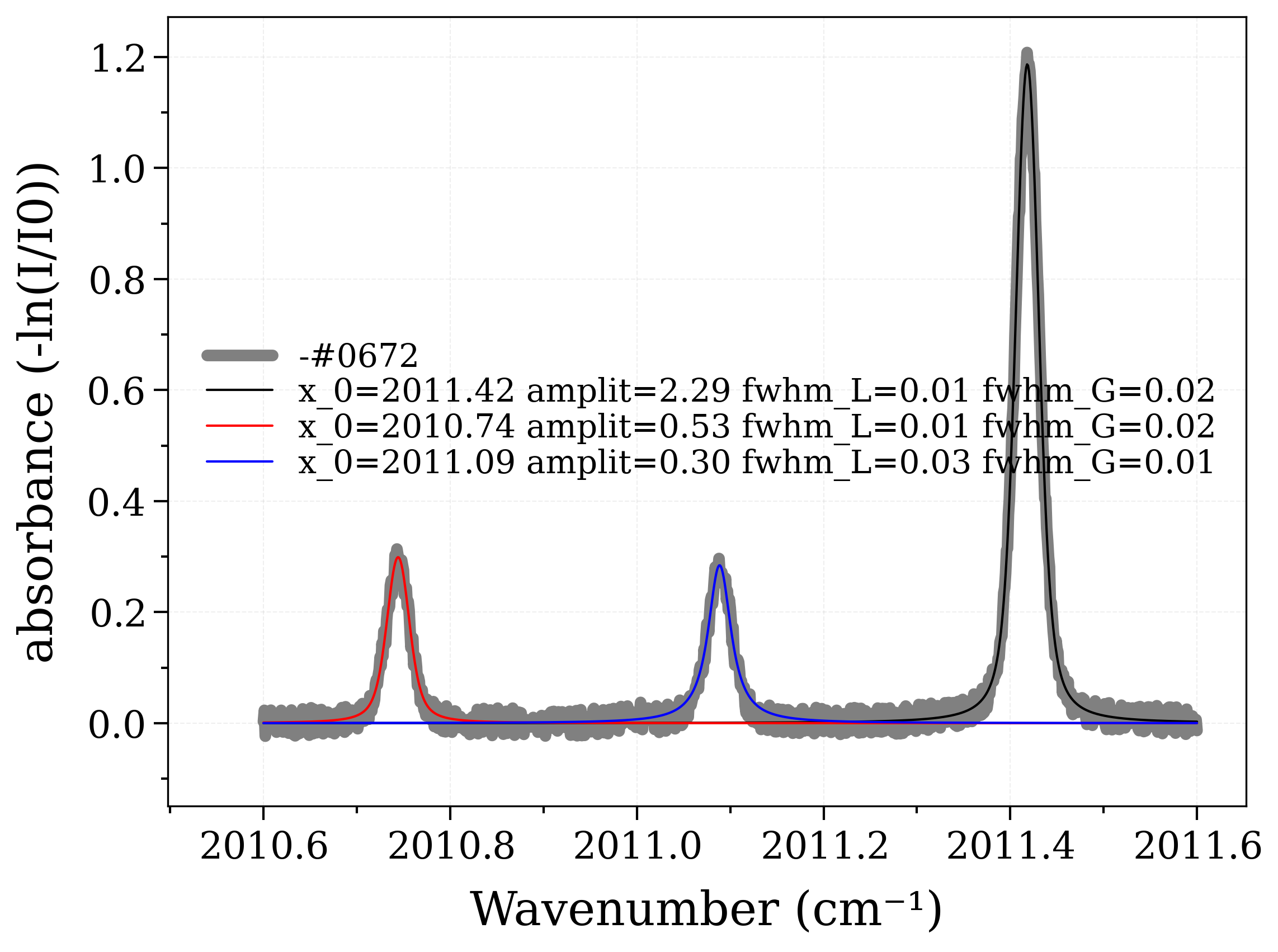
Fit Multiple Voigt Lineshapes

Direct-access functions to fit a sum of three Voigt lineshapes on an experimental spectrum.

This uses the underlying fitting routines of specutils specutils.fitting.fit_lines() routine and some astropy models, among astropy.modeling.functional_models.Gaussian1D, astropy.modeling.functional_models.Lorentz1D or astropy.modeling.functional_models.Voigt1D

import numpy as np

from radis import Spectrum, calc_spectrum
from radis.test.utils import getTestFile

real_experiment = False
if real_experiment:
    T_ref = 7515  # for index 9
    # Using a real experiment (CO in argon) from Minesi et al. (2022) - doi:10.1007/s00340-022-07931-7
    # A warning will be raised because the wavenumber are not evenly spaced (slightly)
    s = Spectrum.from_mat(
        getTestFile("trimmed_1857_VoigtCO_Minesi.mat"),
        "absorbance",
        wunit="cm-1",
        unit="",
        index=9,
    )
else:
    # If using a generated experimental spectrum
    T_ref = 7000
    s = calc_spectrum(
        2010.6,
        2011.6,  # cm-1
        molecule="CO",
        pressure=1,  # bar
        Tgas=T_ref,
        mole_fraction=1,
        path_length=4,
        wstep=0.001,
        databank="hitemp",
        verbose=False,
    )
    w, A = s.get("absorbance")  # extract the wavenumber and absorbance
    noise_amplitude = 5e-2
    rng1 = np.random.default_rng(
        122807528840384100672342137672332424406
    )  # to make sure the fit provides the same output each time
    noise = (
        noise_amplitude * rng1.random(np.size(A)) - noise_amplitude / 2
    )  # simulates the noise of an experiment
    s = Spectrum.from_array(
        w,
        A + noise,
        "absorbance",
        wunit="cm-1",
        unit="",
    )

/home/docs/checkouts/readthedocs.org/user_builds/radis/checkouts/develop/radis/db/molparam.py:252: FutureWarning:

The 'delim_whitespace' keyword in pd.read_csv is deprecated and will be removed in a future version. Use ``sep='\s+'`` instead

from astropy.modeling import models

list_models = [models.Voigt1D() for _ in range(3)]

verbose = False  # verbose=True also recommended
gfit, y_err = s.fit_model(
    list_models, confidence=0.9545, plot=True, verbose=verbose, debug=False
)
if verbose:
    for mod in gfit:
        print(mod)
        print(mod.area)

# Sort models in ascending order of x0
gfit.sort(key=lambda x: x.x_0)

print("-----***********-----\nTemperature fitting:")

-----***********-----
Temperature fitting:

from math import log

E = np.array([17475.8605, 8518.1915, 3378.9537])
S0 = np.array([2.508e-054, 3.206e-036, 3.266e-025])
nu = np.array([2010.746786, 2011.091023, 2011.421043])
name = ["R(8,24)", "R(4,7)", "P(1,25)"]
hc_k = 1.4387752
i0 = 2
T0 = 296
print("-----\nNeglecting stimulated emission:")
for index in [0, 1]:
    R = 1 / (gfit[index].area / gfit[i0].area)
    step = hc_k * (E[index] - E[i0])
    step2 = step / T0
    temp_ratio = step / (
        log(R) + log(S0[index] / S0[i0]) + step2
    )  # see Goldenstein et al. (2016), Eq. 6
    print(
        "Line pair: {0}/{1} \t T = {2:.0f} K, fitting error of {3:.0f}%".format(
            name[index], name[i0], temp_ratio, temp_ratio / T_ref * 100 - 100
        )
    )

-----
Neglecting stimulated emission:
Line pair: R(8,24)/P(1,25)       T = 7057 K, fitting error of 1%
Line pair: R(4,7)/P(1,25)        T = 8373 K, fitting error of 20%

Load HAPI

from radis.db.classes import get_molecule_identifier
from radis.levels.partfunc import PartFuncHAPI

M = get_molecule_identifier("CO")
isotope = 1

Q_HAPI = PartFuncHAPI(M, isotope)
###
T_K = np.arange(100, 8999, 10)
S = np.zeros((3, np.size(T_K)))
for index in [0, 1, 2]:
    num_exp = 1 - np.exp(-hc_k * nu[index] / T_K)
    den_exp = 1 - np.exp(-hc_k * nu[index] / T0)
    S[index] = (
        S0[index]
        * Q_HAPI.at(T0)
        / Q_HAPI.at(list(T_K))
        * np.exp(-hc_k * E[index] * (1 / T_K - 1 / T0))
        * num_exp
        / den_exp
    )

print("-----\nAccounting for stimulated emission:")
for index in [0, 1]:
    R_calc = S[index] / S[i0]
    R_meas = gfit[index].area / gfit[i0].area

    temp_interp = np.interp(R_meas, R_calc, T_K)
    print(
        "Line pair: {0}/{1} \t T = {2:.0f} K, error of {3:.0f}%".format(
            name[index], name[i0], temp_interp, temp_interp / T_ref * 100 - 100
        )
    )

msg = """
**Result**: this fitting routine and the R(8,24)/(P(1,25) line pair
are appropriate for temperature measurement. The R(4,7)/(P(1,25)
line pair requires a more sophiscated fitting routine, due to the
underlying transition at 2011 cm-1 from R(10,115), see Minesi et al. (2022)
"""
print(msg)

-----
Accounting for stimulated emission:
Line pair: R(8,24)/P(1,25)       T = 7058 K, error of 1%
Line pair: R(4,7)/P(1,25)        T = 8374 K, error of 20%

**Result**: this fitting routine and the R(8,24)/(P(1,25) line pair
are appropriate for temperature measurement. The R(4,7)/(P(1,25)
line pair requires a more sophiscated fitting routine, due to the
underlying transition at 2011 cm-1 from R(10,115), see Minesi et al. (2022)

import matplotlib.pyplot as plt for index in [0, 1, 2]:

plt.semilogy(T_K, S[index], label=str(nu[index])) plt.ylim(bottom=1e-24, top=1e-19) plt.xlim(left=2000, right = 9100) plt.legend()