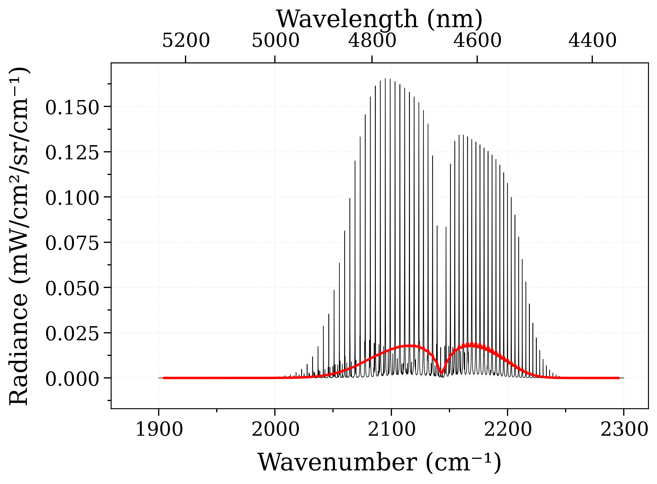
Calculate non-LTE spectra of carbon-monoxide

Compute a CO spectrum with the temperature of the vibrational mode different from the temperature of the rotational mode.

This example uses the calc_spectrum() function, the [HITRAN-2016] line database to derive the line positions and intensities, and the default RADIS spectroscopic constants to compute nonequilibrium energies and populations, but it can be extended to other line databases and other sets of spectroscopic constants.

/home/docs/checkouts/readthedocs.org/user_builds/radis/checkouts/develop/radis/db/molparam.py:252: FutureWarning:

The 'delim_whitespace' keyword in pd.read_csv is deprecated and will be removed in a future version. Use ``sep='\s+'`` instead

Calculating energy levels with Dunham expansion for CO(X1Σ+)(iso1)
Database generated up to v=48, J=238
Calculating energy levels with Dunham expansion for CO(X1Σ+)(iso2)
Database generated up to v=48, J=243
Calculating energy levels with Dunham expansion for CO(X1Σ+)(iso3)
Database generated up to v=48, J=243
Calculating Non-Equilibrium Spectrum
Physical Conditions
----------------------------------------
   Tgas                 300.0 K
   Trot                 300.0 K
   Tvib                 700.0 K
   isotope              1,2,3
   mole_fraction        0.1
   molecule             CO
   path_length          1.0 cm
   pressure             1.01325 bar
   rot_distribution     boltzmann
   self_absorption      True
   state                X
   vib_distribution     boltzmann
   wavenum_max          2300.0000 cm-1
   wavenum_min          1900.0000 cm-1
Computation Parameters
----------------------------------------
   Tref                 296 K
   add_at_used
   broadening_method    voigt
   cutoff               1e-27 cm-1/(#.cm-2)
   dbformat             hitran
   dbpath               /home/docs/.radisdb/hitran/CO.hdf5
   folding_thresh       1e-06
   include_neighbouring_lines  True
   memory_mapping_engine  auto
   neighbour_lines      0 cm-1
   optimization         simple
   parfuncfmt           hapi
   parsum_mode          full summation
   pseudo_continuum_threshold  0
   sparse_ldm           auto
   truncation           50 cm-1
   waveunit             cm-1
   wstep                0.01 cm-1
   zero_padding         -1
----------------------------------------
Fetching Evib & Erot.
/home/docs/checkouts/readthedocs.org/user_builds/radis/checkouts/develop/radis/misc/warning.py:427: NegativeEnergiesWarning:

There are negative rotational energies in the database

/home/docs/checkouts/readthedocs.org/user_builds/radis/checkouts/develop/radis/misc/warning.py:427: PerformanceWarning:

'gu' was recomputed although 'gp' already in DataFrame. All values are equal

... sorting lines by vibrational bands
... lines sorted in 0.0s
Index(['Tdpair', 'A', 'jl', 'vl', 'int', 'iso', 'wav', 'airbrd', 'vu',
       'selbrd', 'gp', 'branch', 'El', 'Pshft', 'ju', 'Eu', 'Evibl', 'Evibu',
       'Erotu', 'Erotl', 'gju', 'gjl', 'grotu', 'grotl', 'gvibu', 'gvibl',
       'gu', 'gl', 'Rs2', 'Blu', 'Bul', 'Aul', 'viblvl_l', 'viblvl_u', 'band'],
      dtype='object')
Index(['Tdpair', 'A', 'jl', 'vl', 'int', 'iso', 'wav', 'airbrd', 'vu',
       'selbrd', 'gp', 'branch', 'El', 'Pshft', 'ju', 'Eu', 'Evibl', 'Evibu',
       'Erotu', 'Erotl', 'gju', 'gjl', 'grotu', 'grotl', 'gvibu', 'gvibl',
       'gu', 'gl', 'Rs2', 'Blu', 'Bul', 'Aul', 'viblvl_l', 'viblvl_u', 'band',
       'Qvib', 'Q', 'Qrotl', 'Qrotu'],
      dtype='object')
Index(['Tdpair', 'A', 'jl', 'vl', 'int', 'iso', 'wav', 'airbrd', 'vu',
       'selbrd', 'gp', 'branch', 'El', 'Pshft', 'ju', 'Eu', 'Evibl', 'Evibu',
       'Erotu', 'Erotl', 'gju', 'gjl', 'grotu', 'grotl', 'gvibu', 'gvibl',
       'gu', 'gl', 'Rs2', 'Blu', 'Bul', 'Aul', 'viblvl_l', 'viblvl_u', 'band',
       'Qvib', 'Q', 'Qrotl', 'Qrotu'],
      dtype='object')
0.20s - Spectrum calculated

<matplotlib.lines.Line2D object at 0x7f30b1f83a30>

from astropy import units as u

from radis import calc_spectrum

s2 = calc_spectrum(
    1900 / u.cm,
    2300 / u.cm,
    molecule="CO",
    isotope="1,2,3",
    pressure=1.01325 * u.bar,
    Tvib=700 * u.K,
    Trot=300 * u.K,
    mole_fraction=0.1,
    path_length=1 * u.cm,
    databank="hitran",  # or use 'hitemp'
)
s2.plot("radiance_noslit")

# Apply a (large) instrumental slit function :
s2.apply_slit(10, "nm")
s2.plot("radiance", nfig="same", lw=2)  # compare with previous