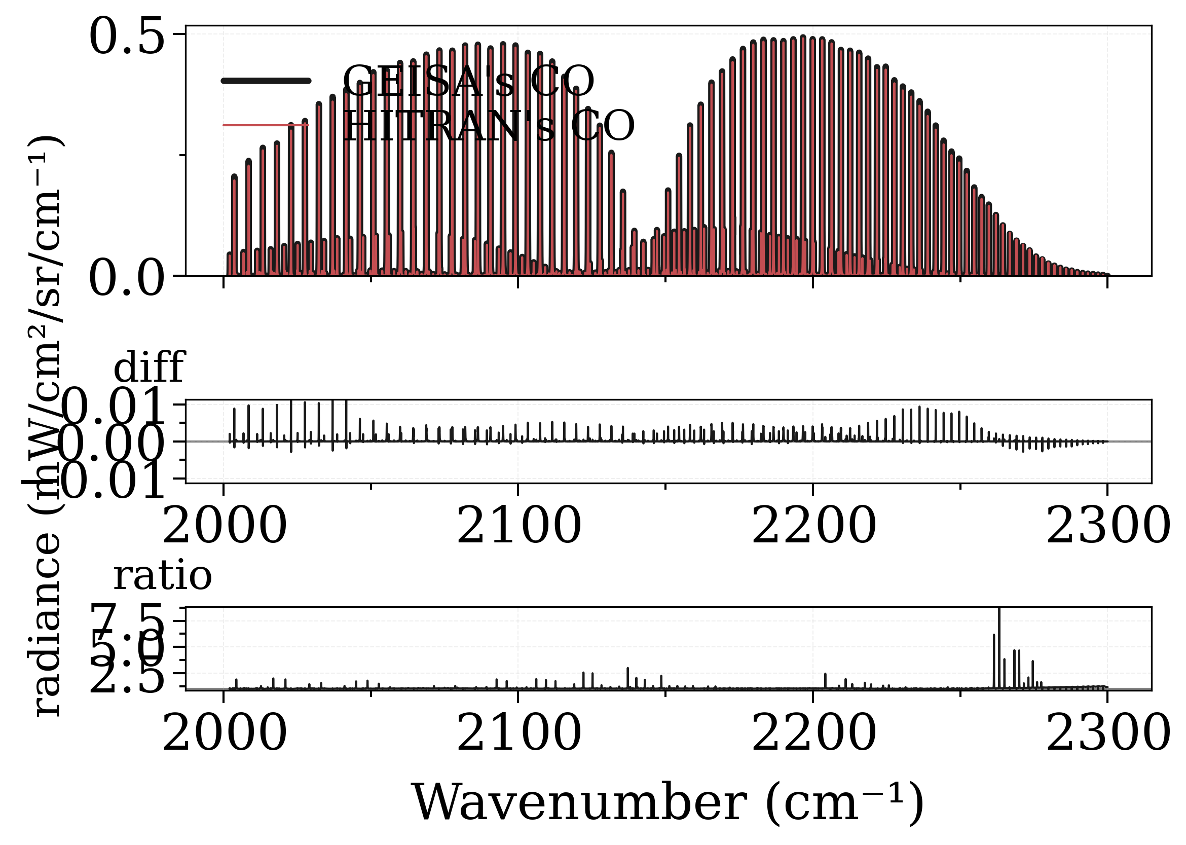
Compare CO spectrum from the GEISA and HITRAN database

GEISA Database has been newly implemented in RADIS 0.13 release on May 15, 2022. This is among the very first attemps to compare the spectra generated from the two databases.

Auto-download and calculate CO spectrum from the GEISA database, and the HITRAN database.

Output should be similar, but not exactly! By default these two databases provide different broadening coefficients. However, the Einstein coefficients & linestrengths should be approximately the same, therefore the integrals under the lines should be similar.

You can see it by running the code below.

For your interest, GEISA and HITRAN lines can be downloaded and accessed separately using fetch_geisa() and fetch_hitran()

Molecule: CO
Downloading line_GEISA2020_asc_gs08_v1.0_co for CO (1/1).
Added GEISA-CO database in /home/docs/radis.json
Calculating Equilibrium Spectrum
Physical Conditions
----------------------------------------
   Tgas                 1000 K
   Trot                 1000 K
   Tvib                 1000 K
   isotope              1,2,3,4,5,6
   mole_fraction        0.1
   molecule             CO
   overpopulation       None
   path_length          1 cm
   pressure_mbar        1013.25 mbar
   rot_distribution     boltzmann
   self_absorption      True
   state                X
   vib_distribution     boltzmann
   wavenum_max          2300.0000 cm-1
   wavenum_min          2002.0000 cm-1
Computation Parameters
----------------------------------------
   Tref                 296 K
   add_at_used
   broadening_method    voigt
   cutoff               1e-27 cm-1/(#.cm-2)
   dbformat             geisa
   dbpath               /home/docs/.radisdb/geisa/CO-line_GEISA2020_asc_gs08_v1.hdf5
   folding_thresh       1e-06
   include_neighbouring_lines  True
   memory_mapping_engine  auto
   neighbour_lines      0 cm-1
   optimization         simple
   parfuncfmt           hapi
   parsum_mode          full summation
   pseudo_continuum_threshold  0
   sparse_ldm           auto
   truncation           50 cm-1
   waveunit             cm-1
   wstep                0.01 cm-1
   zero_padding         -1
----------------------------------------
0.07s - Spectrum calculated
/home/docs/checkouts/readthedocs.org/user_builds/radis/envs/master/lib/python3.8/site-packages/radis/misc/warning.py:354: HighTemperatureWarning:

HITRAN is valid for low temperatures (typically < 700 K). For higher temperatures you may need HITEMP or CDSD. See the 'databank=' parameter

Calculating Equilibrium Spectrum
Physical Conditions
----------------------------------------
   Tgas                 1000 K
   Trot                 1000 K
   Tvib                 1000 K
   isotope              1,2,3,4,5,6
   mole_fraction        0.1
   molecule             CO
   overpopulation       None
   path_length          1 cm
   pressure_mbar        1013.25 mbar
   rot_distribution     boltzmann
   self_absorption      True
   state                X
   vib_distribution     boltzmann
   wavenum_max          2300.0000 cm-1
   wavenum_min          2002.0000 cm-1
Computation Parameters
----------------------------------------
   Tref                 296 K
   add_at_used
   broadening_method    voigt
   cutoff               1e-27 cm-1/(#.cm-2)
   dbformat             hitran
   dbpath               /home/docs/.radisdb/hitran/CO.hdf5
   folding_thresh       1e-06
   include_neighbouring_lines  True
   memory_mapping_engine  auto
   neighbour_lines      0 cm-1
   optimization         simple
   parfuncfmt           hapi
   parsum_mode          full summation
   pseudo_continuum_threshold  0
   sparse_ldm           auto
   truncation           50 cm-1
   waveunit             cm-1
   wstep                0.01 cm-1
   zero_padding         -1
----------------------------------------
0.07s - Spectrum calculated

(<Figure size 640x480 with 3 Axes>, [<AxesSubplot:>, <AxesSubplot:>, <AxesSubplot:xlabel='Wavenumber (cm⁻¹)'>])

import astropy.units as u

from radis import calc_spectrum, plot_diff

conditions = {
    "wmin": 2002 / u.cm,
    "wmax": 2300 / u.cm,
    "molecule": "CO",
    "pressure": 1.01325,  # bar
    "Tgas": 1000,  # K
    "mole_fraction": 0.1,
    "path_length": 1,  # cm
    "verbose": True,
}

s_geisa = calc_spectrum(**conditions, databank="geisa", name="GEISA's CO")

s_hitran = calc_spectrum(
    **conditions,
    databank="hitran",
    name="HITRAN's CO",
)

"""

In :py:func:`~radis.io.geisa.fetch_geisa`, you can choose to additionally plot the
absolute difference (method='diff') by default, or the ratio (method='ratio'), or both.

"""

plot_diff(s_geisa, s_hitran, method=["diff", "ratio"])