Example #3: non-equilibrium spectrum (Tvib, Trot, x_CO)

With the new fitting module introduced in fit_spectrum() function, and in the example of Tgas fitting using new fitting module, we can see its 1-temperature fitting performance for equilibrium condition.

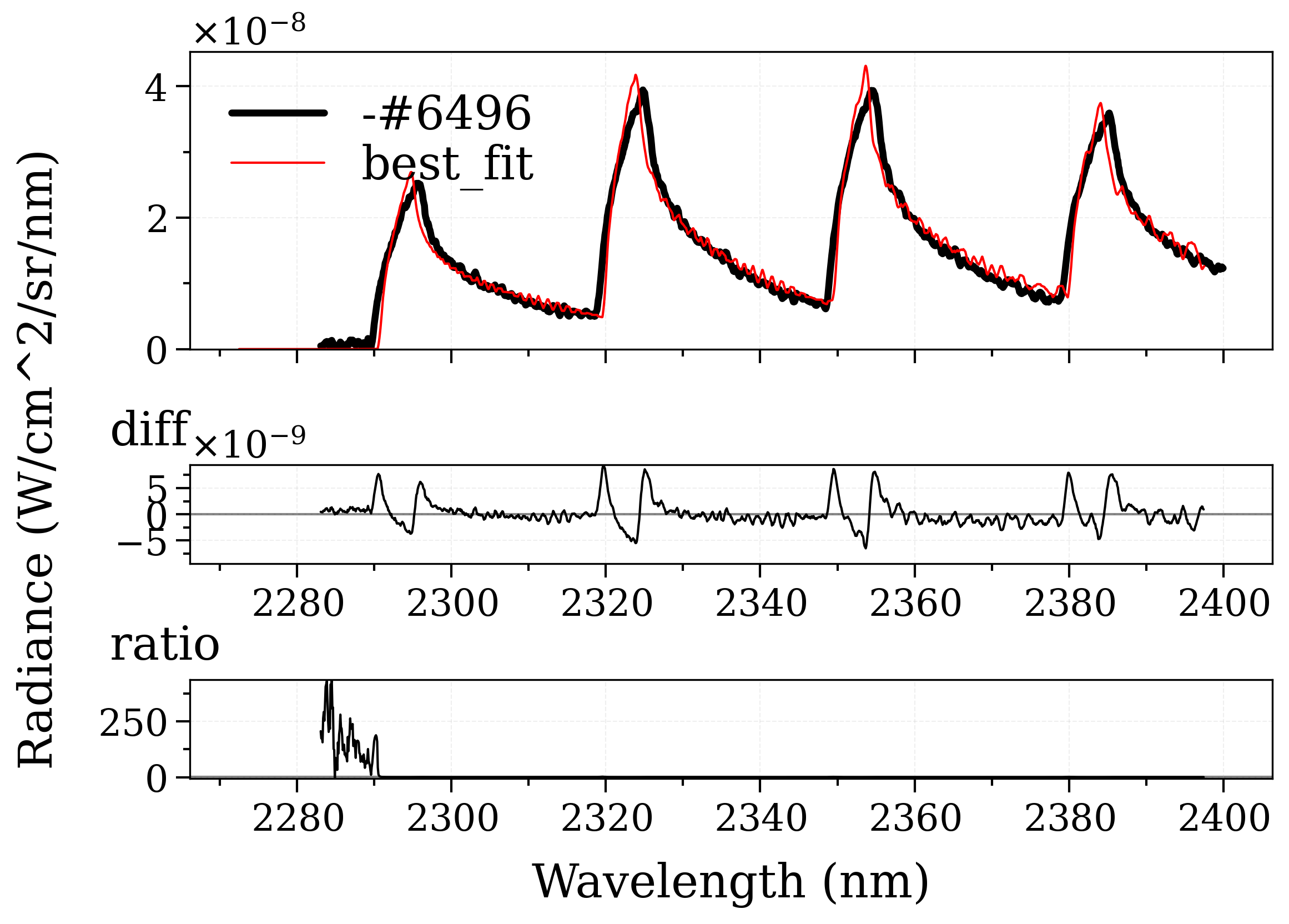
This example features how new fitting module can fit non-equilibrium spectrum, with multiple fit parameters, such as vibrational/rotational temperatures, or mole fraction, etc.

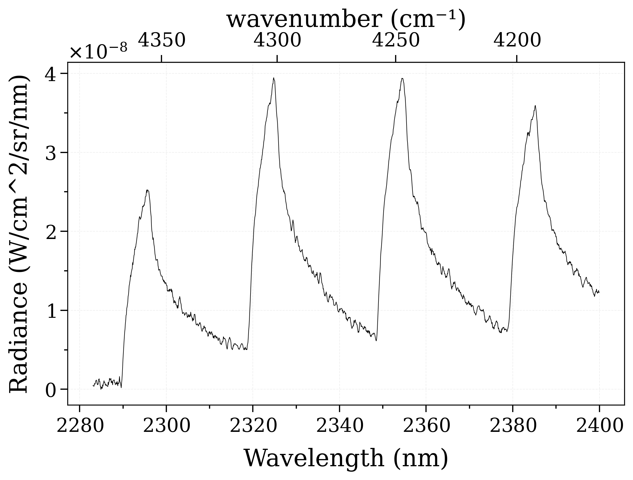
This is a real fitting case introduced Grimaldi’s thesis: https://doi.org/10.2514/1.T6768 . This case features CO molecule emitting on a wide range of spectrum. This case also includes a user-defined trapezoid slit function, which is accounted by the distortion (dispersion) of the slit, as a result of the influences from experimental parameters and spectrometer dispersion parameters during the experiment.

• 
• 

======================= COMMENCE FITTING PROCESS =======================

Successfully retrieved the experimental data in 0.0007793903350830078s.

Acquired spectral quantity 'radiance' from the spectrum.
NaN values successfully purged.Number of data points left: 1479 points.
Successfully refined the experimental data in 0.0002532005310058594s.

Commence fitting process for non-LTE spectrum!
/home/docs/checkouts/readthedocs.org/user_builds/radis/checkouts/master/radis/misc/warning.py:427: PerformanceWarning: 'gu' was recomputed although 'gp' already in DataFrame. All values are equal
  warnings.warn(WarningType(message))
[[Fit Statistics]]
    # fitting method   = L-BFGS-B
    # function evals   = 96
    # data points      = 1
    # variables        = 3
    chi-square         = 4.1191e-21
    reduced chi-square = 4.1191e-21
    Akaike info crit   = -40.9386489
    Bayesian info crit = -46.9386489
##  Warning: uncertainties could not be estimated:
    this fitting method does not natively calculate uncertainties
    and numdifftools is not installed for lmfit to do this. Use
    `pip install numdifftools` for lmfit to estimate uncertainties
    with this fitting method.
[[Variables]]
    Tvib:           4019.23955 (init = 6000)
    Trot:           3213.32472 (init = 4000)
    mole_fraction:  0.06307479 (init = 0.05)

Successfully finished the fitting process in 7.122132062911987s.
/home/docs/checkouts/readthedocs.org/user_builds/radis/checkouts/master/radis/misc/curve.py:240: UserWarning: Presence of NaN in curve_divide!
Think about interpolation=2
  warnings.warn(

======================== END OF FITTING PROCESS ========================


Residual history:

[np.float64(1.6884210236199506e-10), np.float64(1.6884210440381984e-10), np.float64(1.6884210060033468e-10), np.float64(1.6884210671365353e-10), np.float64(3.738560779482434e-10), np.float64(3.738560773031628e-10), np.float64(3.7385607836381597e-10), np.float64(3.738560753446639e-10), np.float64(1.1128815360527545e-10), np.float64(1.1128815379046055e-10), np.float64(1.1128815407823561e-10), np.float64(1.1128815283073891e-10), np.float64(1.0954119407728126e-10), np.float64(1.095411945802535e-10), np.float64(1.0954119427040208e-10), np.float64(1.0954119410263883e-10), np.float64(1.081546823623992e-10), np.float64(1.0815468295021072e-10), np.float64(1.0815468249548762e-10), np.float64(1.0815468255921006e-10), np.float64(1.0308407717343896e-10), np.float64(1.0308407812306925e-10), np.float64(1.0308407707469599e-10), np.float64(1.0308407797781155e-10), np.float64(2.5621875733211255e-10), np.float64(2.562187607828064e-10), np.float64(2.5621875709505406e-10), np.float64(2.5621875666157347e-10), np.float64(9.533543779641823e-11), np.float64(9.533543905716837e-11), np.float64(9.53354375654258e-11), np.float64(9.533543887685615e-11), np.float64(8.484273770465598e-11), np.float64(8.484273907398177e-11), np.float64(8.484273746993825e-11), np.float64(8.48427386753232e-11), np.float64(2.9421697749802616e-10), np.float64(2.942169743129064e-10), np.float64(2.942169781660324e-10), np.float64(2.942169764324424e-10), np.float64(7.54577676798936e-11), np.float64(7.545776870127448e-11), np.float64(7.545776760904074e-11), np.float64(7.545776813893211e-11), np.float64(6.932653661965616e-11), np.float64(6.932653524859567e-11), np.float64(6.932653726881375e-11), np.float64(6.932653526306025e-11), np.float64(7.949285617556162e-11), np.float64(7.94928575693033e-11), np.float64(7.94928559076233e-11), np.float64(7.949285708515032e-11), np.float64(6.814984172976307e-11), np.float64(6.814984119330466e-11), np.float64(6.814984214615076e-11), np.float64(6.814984090177898e-11), np.float64(6.719214631439374e-11), np.float64(6.719214592190663e-11), np.float64(6.719214660971042e-11), np.float64(6.719214565247127e-11), np.float64(6.549162026237408e-11), np.float64(6.549162024921514e-11), np.float64(6.549162014368664e-11), np.float64(6.549162007021926e-11), np.float64(6.525776580881548e-11), np.float64(6.525776582002855e-11), np.float64(6.525776567740905e-11), np.float64(6.525776565981386e-11), np.float64(6.42332113641256e-11), np.float64(6.423321122577801e-11), np.float64(6.423321137797768e-11), np.float64(6.423321126693566e-11), np.float64(6.418825478779295e-11), np.float64(6.418825486312706e-11), np.float64(6.418825476634321e-11), np.float64(6.41882548252725e-11), np.float64(6.418046442464562e-11), np.float64(6.41804644162452e-11), np.float64(6.418046442991702e-11), np.float64(6.418046441969829e-11), np.float64(6.41803383933946e-11), np.float64(6.418033839175417e-11), np.float64(6.418033839463874e-11), np.float64(6.418033839184987e-11), np.float64(6.418032597713388e-11), np.float64(6.418032597680558e-11), np.float64(6.418032597745491e-11), np.float64(6.418032597667379e-11), np.float64(6.418032367206444e-11), np.float64(6.418032367210007e-11), np.float64(6.418032367204727e-11), np.float64(6.418032367207604e-11), np.float64(6.418032366726713e-11), np.float64(6.418032366727015e-11), np.float64(6.418032366726541e-11), np.float64(6.418032366726866e-11), np.float64(6.418032366726713e-11)]

Fitted values history:

[6000.0, 4000.0, 0.05]
[6000.00002, 4000.0, 0.05]
[6000.0, 4000.000024494898, 0.05]
[6000.0, 4000.0, 0.0500000005]
[5105.589010335032, 4855.661718393352, 0.012435519473900064]
[5105.589034590468, 4855.661718393352, 0.012435519473900064]
[5105.589010335032, 4855.66174313907, 0.012435519473900064]
[5105.589010335032, 4855.661718393352, 0.012435519803886397]
[5818.190228771631, 4187.474367180093, 0.04066587321110825]
[5818.190250013982, 4187.474367180093, 0.04066587321110825]
[5818.190228771631, 4187.47439198398, 0.04066587321110825]
[5818.190228771631, 4187.474367180093, 0.04066587370231839]
[5807.1648517841895, 4147.480389673976, 0.0419975752938115]
[5807.164873094562, 4147.480389673976, 0.0419975752938115]
[5807.1648517841895, 4147.480414424188, 0.0419975752938115]
[5807.1648517841895, 4147.480389673976, 0.04199757578736607]
[5757.359696234136, 4111.453804699595, 0.042512311868348265]
[5757.359717842112, 4111.453804699595, 0.042512311868348265]
[5757.359696234136, 4111.453829395813, 0.042512311868348265]
[5757.359696234136, 4111.453804699595, 0.04251231236270993]
[5551.640602378711, 3968.248691625253, 0.044578828600610916]
[5551.640625059214, 3968.248691625253, 0.044578828600610916]
[5551.640602378711, 3968.2487160531887, 0.044578828600610916]
[5551.640602378711, 3968.248691625253, 0.044578829097663315]
[2363.258906498787, 2028.0365503627763, 0.08815012505490516]
[2363.258893520584, 2028.0365503627763, 0.08815012505490516]
[2363.258906498787, 2028.0365466291896, 0.08815012505490516]
[2363.258906498787, 2028.0365503627763, 0.08815012537810292]
[5270.459855349492, 3795.364451309296, 0.046884237967710636]
[5270.459879132662, 3795.364451309296, 0.046884237967710636]
[5270.459855349492, 3795.3644752957266, 0.046884237967710636]
[5270.459855349492, 3795.364451309296, 0.04688423846673889]
[4949.512393747401, 3610.0308913631948, 0.049418549258804734]
[4949.5124183399585, 3610.0308913631948, 0.049418549258804734]
[4949.512393747401, 3610.0309147254616, 0.049418549258804734]
[4949.512393747401, 3610.0308913631948, 0.04941854975877092]
[2440.730670951443, 2341.0394159153043, 0.07075979316396933]
[2440.7306851268086, 2341.0394159153043, 0.07075979316396933]
[2440.730670951443, 2341.0394285204193, 0.07075979316396933]
[2440.730670951443, 2341.0394159153043, 0.07075979361883536]
[4677.68364067358, 3460.716773535213, 0.05151739148765927]
[4677.683665610357, 3460.716773535213, 0.05151739148765927]
[4677.68364067358, 3460.716796272606, 0.05151739148765927]
[4677.68364067358, 3460.716773535213, 0.051517391987428975]
[4198.139731846036, 3209.9159649686617, 0.05518698394224544]
[4198.139756663128, 3209.9159649686617, 0.05518698394224544]
[4198.139731846036, 3209.91598638287, 0.05518698394224544]
[4198.139731846036, 3209.9159649686617, 0.055186984439547684]
[4786.934731711908, 3491.1877412664817, 0.0507318508130918]
[4786.9347565467, 3491.1877412664817, 0.0507318508130918]
[4786.934731711908, 3491.187764140698, 0.0507318508130918]
[4786.934731711908, 3491.1877412664817, 0.05073185131303823]
[4316.412760333622, 3265.0317905576635, 0.054292006570630526]
[4316.412785266122, 3265.0317905576635, 0.054292006570630526]
[4316.412760333622, 3265.031812294392, 0.054292006570630526]
[4316.412760333622, 3265.0317905576635, 0.05429200706878499]
[4284.4043846550685, 3228.8457755549384, 0.05493288553095069]
[4284.404409561932, 3228.8457755549384, 0.05493288553095069]
[4284.4043846550685, 3228.8457970820537, 0.05493288553095069]
[4284.4043846550685, 3228.8457755549384, 0.05493288602851139]
[4145.561510048648, 3098.522621578824, 0.05762044312738075]
[4145.561534796119, 3098.522621578824, 0.05762044312738075]
[4145.561510048648, 3098.5226422811456, 0.05762044312738075]
[4145.561510048648, 3098.522621578824, 0.05762044362153951]
[4126.632888218992, 3101.825145312422, 0.05824217707545718]
[4126.632912938614, 3101.825145312422, 0.05824217707545718]
[4126.632888218992, 3101.8251660370624, 0.05824217707545718]
[4126.632888218992, 3101.825145312422, 0.05824217756861705]
[4017.831776104892, 3184.582033973548, 0.06249110875070785]
[4017.831800635513, 3184.582033973548, 0.06249110875070785]
[4017.831776104892, 3184.582055233076, 0.06249110875070785]
[4017.831776104892, 3184.582033973548, 0.06249110923485371]
[4030.630355300628, 3216.4133792192188, 0.06286712412691618]
[4030.6303798560593, 3216.4133792192188, 0.06286712412691618]
[4030.630355300628, 3216.413400672436, 0.06286712412691618]
[4030.630355300628, 3216.4133792192188, 0.0628671246100763]
[4019.035074189604, 3214.762390960352, 0.06308863084988077]
[4019.0350987225875, 3214.762390960352, 0.06308863084988077]
[4019.035074189604, 3214.762412403683, 0.06308863084988077]
[4019.035074189604, 3214.762390960352, 0.06308863133244556]
[4019.7015375870724, 3213.618094126655, 0.06306124494443911]
[4019.7015621213613, 3213.618094126655, 0.06306124494443911]
[4019.7015375870724, 3213.618115563123, 0.06306124494443911]
[4019.7015375870724, 3213.618094126655, 0.0630612454270781]
[4019.4652380984885, 3213.397911448943, 0.06306791859457209]
[4019.4652626323145, 3213.397911448943, 0.06306791859457209]
[4019.4652380984885, 3213.3979328840896, 0.06306791859457209]
[4019.4652380984885, 3213.397911448943, 0.063067919077193]
[4019.248493923078, 3213.3204521369044, 0.06307448334325043]
[4019.2485184564794, 3213.3204521369044, 0.06307448334325043]
[4019.248493923078, 3213.320473571586, 0.06307448334325043]
[4019.248493923078, 3213.3204521369044, 0.06307448382585355]
[4019.2395520501627, 3213.3247220926482, 0.06307478507965011]
[4019.239576583547, 3213.3247220926482, 0.06307478507965011]
[4019.2395520501627, 3213.3247435273556, 0.06307478507965011]
[4019.2395520501627, 3213.3247220926482, 0.06307478556225243]
[4019.2395520501627, 3213.3247220926482, 0.06307478507965011]

Total fitting time:
7.122132062911987 s

import astropy.units as u
import numpy as np

from radis import load_spec
from radis.test.utils import getTestFile
from radis.tools.new_fitting import fit_spectrum

# The following function and parameters reproduce the slit function in Dr. Corenti Grimaldi's thesis.


def slit_dispersion(w):
    phi = -6.33
    f = 750
    gr = 300
    m = 1
    phi *= -2 * np.pi / 360
    d = 1e-3 / gr
    disp = (
        w
        / (2 * f)
        * (-np.tan(phi) + np.sqrt((2 * d / m / (w * 1e-9) * np.cos(phi)) ** 2 - 1))
    )
    return disp  # nm/mm


slit = 1500  # µm
pitch = 20  # µm
top_slit_um = slit - pitch  # µm
base_slit_um = slit + pitch  # µm
center_slit = 5090
dispersion = slit_dispersion(center_slit)
top_slit_nm = top_slit_um * 1e-3 * dispersion
base_slit_nm = base_slit_um * 1e-3 * dispersion * 1.33


# -------------------- Step 1. Load experimental spectrum -------------------- #


specName = (
    "Corentin_0_100cm_DownSampled_20cm_10pctCO2_1-wc-gw450-gr300-sl1500-acc5000-.spec"
)
s_experimental = load_spec(getTestFile(specName)).offset(-0.6, "nm")


# -------------------- Step 2. Fill ground-truths and data -------------------- #


# Experimental conditions which will be used for spectrum modeling. Basically, these are known ground-truths.
experimental_conditions = {
    "molecule": "CO",  # Molecule ID
    "isotope": "1,2,3",  # Isotope ID, can have multiple at once
    "wmin": 2270
    * u.nm,  # Starting wavelength/wavenumber to be cropped out from the original experimental spectrum.
    "wmax": 2400 * u.nm,  # Ending wavelength/wavenumber for the cropping range.
    "pressure": 1.01325
    * u.bar,  # Total pressure of gas, in "bar" unit by default, but you can also use Astropy units.
    "path_length": 1
    / 195
    * u.cm,  # Experimental path length, in "cm" unit by default, but you can also use Astropy units.
    "slit": {  # Experimental slit. In simple form: "[value] [unit]", i.e. "-0.2 nm". In complex form: a dict with parameters of apply_slit()
        "slit_function": (top_slit_nm, base_slit_nm),
        "unit": "nm",
        "shape": "trapezoidal",
        "center_wavespace": center_slit,
        "slit_dispersion": slit_dispersion,
        "inplace": False,
    },
    "cutoff": 0,  # (RADIS native) Discard linestrengths that are lower that this to reduce calculation time, in cm-1.
    "databank": "hitemp",  # Databank used for calculation. Must be stated.
}

# List of parameters to be fitted, accompanied by its initial value
fit_parameters = {
    "Tvib": 6000,  # Vibrational temperature, in K.
    "Trot": 4000,  # Rotational temperature, in K.
    "mole_fraction": 0.05,  # Species mole fraction, from 0 to 1.
}

# List of bounding ranges applied for those fit parameters above.
# You can skip this step and let it use default bounding ranges, but this is not recommended.
# Bounding range must be at format [<lower bound>, <upper bound>].
bounding_ranges = {
    "Tvib": [2000, 7000],
    "Trot": [2000, 7000],
    "mole_fraction": [0, 0.1],
}

# Fitting pipeline setups.
fit_properties = {
    "method": "lbfgsb",  # Preferred fitting method. By default, "leastsq".
    "fit_var": "radiance",  # Spectral quantity to be extracted for fitting process, such as "radiance", "absorbance", etc.
    "normalize": False,  # Either applying normalization on both spectra or not.
    "max_loop": 300,  # Max number of loops allowed. By default, 200.
    "tol": 1e-20,  # Fitting tolerance, only applicable for "lbfgsb" method.
}

"""

For the fitting method, you can try one among 17 different fitting methods and algorithms of LMFIT,
introduced in `LMFIT method list <https://lmfit.github.io/lmfit-py/fitting.html#choosing-different-fitting-methods>`.

You can see the benchmark result of these algorithms here:
`RADIS Newfitting Algorithm Benchmark <https://github.com/radis/radis-benchmark/blob/master/manual_benchmarks/plot_newfitting_comparison_algorithm.py>`.

"""


# -------------------- Step 3. Run the fitting and retrieve results -------------------- #

# Conduct the fitting process!
s_best, result, log = fit_spectrum(
    s_exp=s_experimental,  # Experimental spectrum.
    fit_params=fit_parameters,  # Fit parameters.
    bounds=bounding_ranges,  # Bounding ranges for those fit parameters.
    model=experimental_conditions,  # Experimental ground-truths conditions.
    pipeline=fit_properties,  # # Fitting pipeline references.
)

# Now investigate the result logs for additional information about what's going on during the fitting process

print("\nResidual history: \n")
print(log["residual"])

print("\nFitted values history: \n")
for fit_val in log["fit_vals"]:
    print(fit_val)

print("\nTotal fitting time: ")
print(log["time_fitting"], end=" s\n")