Example #1: Temperature fit

RADIS has its own fitting feature, as shown in 1 temperature fit example, where you have to manually create the spectrum model, input the experimental spectrum and other ground-truths into numerous RADIS native functions, and adjust the fitting pipeline yourself.

Now with the new fitting module released, all you have to do is to prepare a .spec file containing your experimental spectrum, fill some JSON forms describing the ground-truth conditions just like how you fill a medical checkup paper, call the function fit_spectrum() and let it do all the work! If you are not satisfied with the result, you can simply adjust the parameters in your JSON such as slit and path_length, recall the function until the results are good.

Instruction:

• Step 1: prepare a .spec file. Create a .spec file containing your experimental spectrum. You can do it with RADIS by saving a Spectrum object with store(). If your current data is not a Spectrum object, you can convert it to a Spectrum object from Python arrays or from text files, and then save it as .spec file as above.

• Step 2: fill the JSON forms. There are 4 JSON forms you need to fill: experimental_conditions with ground-truth data about your experimental environment, fit_parameters with the parameters you need to fit (such as Tgas, mole fraction, etc.), bounding_ranges with fitting ranges for parameters you listed in fit_parameters, and fit_properties for some fitting pipeline references.

• Step 3: call fit_spectrum() with the experimental spectrum and 4 JSON forms, then see the result.

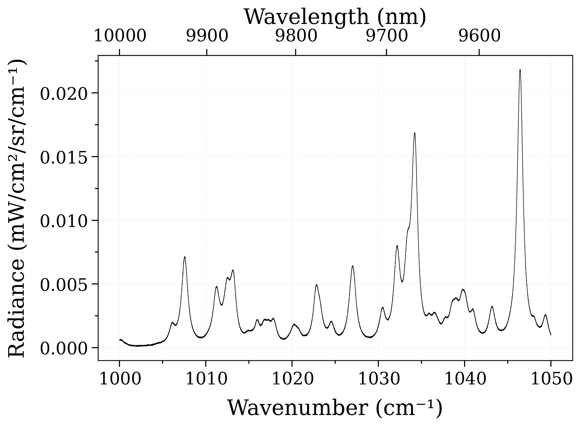
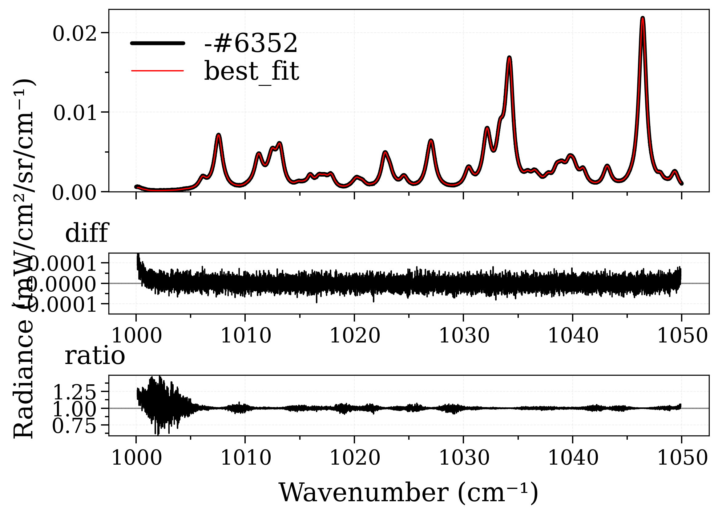
This example features fitting an experimental spectrum with Tgas, using new fitting modules.

• 
• 

======================= COMMENCE FITTING PROCESS =======================

Successfully retrieved the experimental data in 0.0008828639984130859s.

Acquired spectral quantity 'radiance' from the spectrum.
NaN values successfully purged.Number of data points left: 16666 points.
Successfully refined the experimental data in 0.0005700588226318359s.
"tol" parameter spotted but "method" is not "lbfgsb"!
Added HITRAN-NH3 database in /home/docs/radis.json

Commence fitting process for LTE spectrum!

[[Fit Statistics]]
    # fitting method   = least_squares
    # function evals   = 16
    # data points      = 1
    # variables        = 1
    chi-square         = 8.9703e-14
    reduced chi-square = 8.9703e-14
    Akaike info crit   = -28.0422690
    Bayesian info crit = -30.0422690
[[Variables]]
    Tgas:  1000.00489 +/- 99.8567109 (9.99%) (init = 700)

Successfully finished the fitting process in 4.480479717254639s.
/home/docs/checkouts/readthedocs.org/user_builds/radis/checkouts/master/radis/misc/curve.py:267: UserWarning: First spectrum has more resolution than 2nd. Reverse your spectra in interpolation/comparison for a better accuracy
  warnings.warn(
/home/docs/checkouts/readthedocs.org/user_builds/radis/checkouts/master/radis/misc/curve.py:267: UserWarning: First spectrum has more resolution than 2nd. Reverse your spectra in interpolation/comparison for a better accuracy
  warnings.warn(
/home/docs/checkouts/readthedocs.org/user_builds/radis/checkouts/master/radis/misc/curve.py:240: UserWarning: Presence of NaN in curve_divide!
Think about interpolation=2
  warnings.warn(

======================== END OF FITTING PROCESS ========================


Residual history:

[np.float64(2.2247874224512415e-05), np.float64(2.2247873785034496e-05), np.float64(6.253348055219789e-06), np.float64(6.253349349508807e-06), np.float64(6.72028146816917e-07), np.float64(6.720292786352701e-07), np.float64(3.2924634954483526e-07), np.float64(3.292458258119761e-07), np.float64(7.106633722253802e-07), np.float64(3.049825797614543e-07), np.float64(3.049828213445954e-07), np.float64(3.097819889163911e-07), np.float64(3.0027155195651623e-07), np.float64(3.002716522956089e-07), np.float64(2.9950506491289325e-07), np.float64(2.995050202189005e-07), np.float64(2.9950506491289325e-07)]

Fitted values history:

[700.0]
[700.0000104308128]
[1075.5142877173294]
[1075.514303743741]
[1007.2652361151856]
[1007.2652511246073]
[998.5071149334882]
[998.5071298124037]
[1007.7742406227084]
[1000.8238963557932]
[1000.8239112692314]
[999.1855578098264]
[1000.4143117193015]
[1000.4143266266365]
[1000.004894600663]
[1000.0049095018971]
[1000.004894600663]

Total fitting time:
4.480479717254639 s

import astropy.units as u

from radis import load_spec
from radis.test.utils import getTestFile
from radis.tools.new_fitting import fit_spectrum

# -------------------- Step 1. Load experimental spectrum -------------------- #

# Load an experimental spectrum. You can prepare yours, or fetch one of them in the radis/test/files directory.
my_spec = getTestFile("synth-NH3-1-500-2000cm-P10-mf0.01-p1.spec")
s_experimental = load_spec(my_spec)


# -------------------- Step 2. Fill ground-truths and data -------------------- #

# Experimental conditions which will be used for spectrum modeling. Basically, these are known ground-truths.
experimental_conditions = {
    "molecule": "NH3",  # Molecule ID
    "isotope": "1",  # Isotopologue - also "all" or "1,2"
    "wmin": 1000,  # Starting wavelength/wavenumber to be cropped out from the original experimental spectrum.
    "wmax": 1050,  # Ending wavelength/wavenumber for the cropping range.
    "wunit": "cm-1",  # Unit of "wmin"/"wmax"
    "mole_fraction": 0.01,  # Species mole fraction, from 0 to 1.
    "pressure": 1e6
    * u.Pa,  # Total pressure of gas, in "bar" unit by default, but you can also use Astropy units.
    "path_length": 10
    * u.mm,  # Experimental path length, in "cm" unit by default, but you can also use Astropy units.
    "slit": "1 nm",  # Experimental slit, must be a blank space separating slit amount and unit.
    "offset": "-0.2 nm",  # Experimental offset, must be a blank space separating offset amount and unit.
    "databank": "hitran",  # Databank used for the spectrum calculation. Must be stated.
}

# List of parameters to be fitted, accompanied by their initial values.
# Comment : an initial parameter too far from reality will impede convergence
fit_parameters = {
    "Tgas": 700,  # Gas temperature, in K.
}

# List of bounding ranges applied for those fit parameters above.
# You can skip this step and let it use default bounding ranges, but this is not recommended.
# Bounding range must be at format [<lower bound>, <upper bound>].
bounding_ranges = {
    "Tgas": [500, 2000],
}

# Fitting pipeline setups.
fit_properties = {
    "method": "least_squares",  # Preferred fitting method from the 17 confirmed methods of LMFIT stated in week 4 blog. By default, "leastsq".
    "fit_var": "radiance",  # Spectral quantity to be extracted for fitting process, such as "radiance", "absorbance", etc.
    "normalize": False,  # Either applying normalization on both spectra or not.
    "max_loop": 150,  # Max number of loops allowed. By default, 200.
    "tol": 1e-15,  # Fitting tolerance, only applicable for "lbfgsb" method.
}

"""

For the fitting method, you can try one among 17 different fitting methods and algorithms of LMFIT,
introduced in `LMFIT method list <https://lmfit.github.io/lmfit-py/fitting.html#choosing-different-fitting-methods>`.

You can see the benchmark result of these algorithms here:
`RADIS Newfitting Algorithm Benchmark <https://github.com/radis/radis-benchmark/blob/master/manual_benchmarks/plot_newfitting_comparison_algorithm.py>`.

"""


# -------------------- Step 3. Run the fitting and retrieve results -------------------- #


# Conduct the fitting process!
s_best, result, log = fit_spectrum(
    s_exp=s_experimental,  # Experimental spectrum.
    fit_params=fit_parameters,  # Fit parameters.
    bounds=bounding_ranges,  # Bounding ranges for those fit parameters.
    model=experimental_conditions,  # Experimental ground-truths conditions.
    pipeline=fit_properties,  # Fitting pipeline references.
    fit_kws={"gtol": 1e-12},
)


# Now investigate the result logs for additional information about what's going on during the fitting process

print("\nResidual history: \n")
print(log["residual"])

print("\nFitted values history: \n")
for fit_val in log["fit_vals"]:
    print(fit_val)

print("\nTotal fitting time: ")
print(log["time_fitting"], end=" s\n")